


[This lecture was partially created with the support of Artificial Intelligence tools (ChatGPT)]
1. Introduction
Deterministic models play a central role in environmental science by providing a structured and theory-driven way to estimate, predict, and understand environmental variables. At their core, deterministic models are based on the assumption that the behavior of a system can be fully described by a set of known relationships, typically expressed through mathematical equations derived from physical, chemical, or biological principles. Unlike stochastic approaches, which explicitly incorporate randomness and uncertainty, deterministic models produce a single, reproducible output for a given set of inputs and parameters. This characteristic makes them particularly valuable for exploring cause–effect relationships and for testing hypotheses about how environmental systems respond to changes in external conditions.
In applications, deterministic models are widely used to estimate variables such as air pollutant concentrations, water quality indicators, soil moisture, and ecosystem productivity. For example, atmospheric dispersion models simulate how pollutants emitted from a source are transported and diluted in the atmosphere based on wind speed, turbulence, and chemical reactions. Similarly, hydrological models estimate river discharge or groundwater levels by representing processes such as precipitation, infiltration, evapotranspiration, and runoff. These models are typically built upon conservation laws, such as the conservation of mass or energy, and are implemented through differential or algebraic equations that describe how environmental variables evolve over space and time.
One of the key strengths of deterministic models lies in their interpretability. Because they are grounded in established scientific laws, their structure provides insight into the mechanisms driving environmental processes. This makes them especially useful for scenario analysis, where researchers and policymakers assess the potential impacts of interventions such as emission reductions, land-use changes, or climate variability. By systematically adjusting input variables, deterministic models can help identify critical thresholds, sensitivities, and feedbacks within environmental systems.
In recent years, deterministic models have increasingly been integrated with data-driven and probabilistic approaches to improve their robustness and predictive power. Hybrid frameworks, for instance, combine physically based equations with statistical or machine learning components to better capture complex dynamics and reduce biases. Despite these advances, deterministic modeling remains a foundational tool in environmental analysis, providing a coherent framework for synthesizing scientific knowledge and supporting evidence-based decision making.
Understanding deterministic models involves not only learning the mathematical formulations and computational techniques but also developing a critical awareness of their assumptions, limitations, and appropriate domains of application. When used thoughtfully, deterministic models offer powerful insights into environmental systems and serve as an essential bridge between theoretical understanding and real-world problem solving.
Definition of deterministic model
A deterministic model produces the same output from a given starting condition or initial state, because no randomness is involved.
The output from a deterministic model may include a single variables or multiple variables, which are unknown. In particular, a deterministic model may produce a single output, like the peak flow or peak wind speed for a certain location, or multiple variables at different locations, or a sequence along space or along time of the same variable. An example is the prediction of rainfall along time for a certain location, therefore predicting what we call a "process", namely, the dynamics along time (or along space) of a given phenomena, which we observe by measuring a variable.
Additionally, the model may include additional unknown dynamic variables that are essential for describing the state of the system. These are called "state variables" and may be also unknown.
A deterministic model is typically given by a system of equations relating input variables, state variables and output variables. The number of equations is at least equivalent to the number of unknowns. Equations may be physically-based, or chemically-based, or based on other theories governing the evolution of the process. In alternative, equations may be empirical.
2. Added value of deterministic models
Deterministic models do not account for randomness and therefore are computationally more efficient with respect to solutions accounting for randomness and uncertainty. Therefore, deterministic models are often preferred for the representation of complex systems. Being based on a theoretically based description of the system, deterministic models are transparent and look rigorous in their representation.
Furthermore, being based on a rigorous representation of the system, deterministic model can be in principle applied without calibration and therefore deliver solutions to overcome the challenge of lack of observed data, which are instead essential for the application of data driven approaches. For instance, in absence of observed river flow, these can be reconstructed by routing rainfall data and other meteorological variables through a rainfall-runoff model.
3. Limitations of deterministic models
Deterministic models produce a single output from a given set of inputs based on fixed equations. Their applicability is constrained by several important limitations. First, they rely heavily on the completeness and accuracy of the underlying process representation. Environmental systems are inherently complex, often involving nonlinear interactions, spatial heterogeneity, processes that are difficult to measure directly, and often only partially understood. Thus, deterministic formulations inevitably simplify or omit processes, leading to structural model error. Second, input data uncertainty propagates directly into outputs. Measurements of environmental variables (e.g., emissions, boundary conditions, land use) are often sparse, noisy, or biased, yet deterministic models typically do not explicitly account for this uncertainty, giving a false sense of precision.
As a result, deterministic models require simplifying assumptions and parameterizations, which can introduce uncertainty and limit their accuracy.
Second, parameter estimation poses a critical challenge. Many environmental models include parameters that cannot be directly measured and must be calibrated, often resulting in equifinality—different parameter sets producing similar outputs—thereby reducing interpretability and predictive robustness. Model calibration and validation are therefore essential steps, involving the adjustment of model parameters to match observed data and the evaluation of model performance against independent datasets. Even though deterministic models do not explicitly include randomness, uncertainty still arises from imperfect knowledge of inputs, parameters, and system structure.
Third, deterministic models struggle to capture stochastic variability and extreme events, which are intrinsic to environmental systems (e.g., sudden storms, ecological disturbances). This limits their reliability, particularly for risk assessment and decision-making under uncertainty.
Finally, scale mismatches (temporal and spatial) between model structure and real-world processes can introduce systematic biases. Finally, deterministic models can be computationally expensive when representing high-resolution systems, restricting their use in large-scale or real-time applications. For these reasons, probabilistic, stochastic, or hybrid modeling approaches are often preferred to complement deterministic frameworks and better represent uncertainty and variability.
Box: non-linearity and chaos
Nonlinearity refers to systems in which outputs are not proportional to inputs, meaning small changes can produce disproportionately large or complex effects. In environmental and physical systems, this often arises from feedback loops, thresholds, and interactions among multiple components. Because of nonlinearity, such systems cannot be accurately described by simple additive relationships, and their behavior may change qualitatively across different conditions.
Chaos is a property of certain nonlinear dynamical systems characterized by extreme sensitivity to initial conditions, often summarized as the “butterfly effect.” Even infinitesimally small differences in starting states can lead to vastly different trajectories over time, making long-term prediction inherently difficult despite the system being deterministic. Chaotic systems are not random, but they appear irregular and unpredictable due to this sensitivity. Together, nonlinearity and chaos explain why many natural systems—such as climate, ecosystems, and fluid dynamics—exhibit complex, evolving patterns that challenge precise prediction.
4. A first meaningful example: climate models
Climate models (see here for more details) and meteorological models are meaningful examples of deterministic models. They describe with deterministic relationships the dynamics of climate and meteorological processes by typically relying on conservation equations applied at the grid scale (see Figure below). By feeding these models with proper initial and boundary conditions, and assigned scenarios of future emissions for climate models, these models deliver projections of future climate and meteorological predictions.
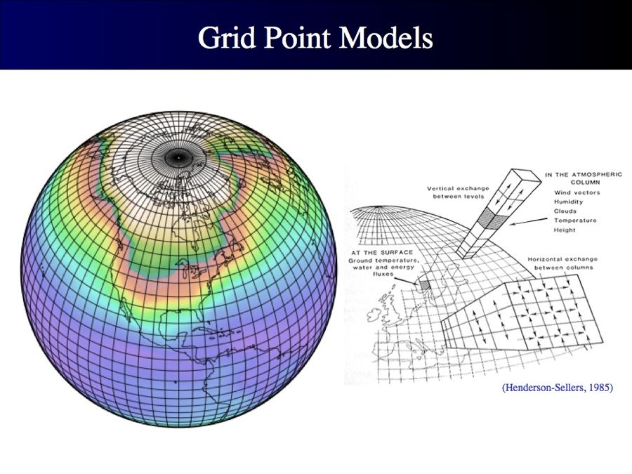
Figure 1. Grid scale representation of climate models. Source: https://www.nccs.nasa.gov/services/climate-data-services.
In a single model run of climate models, there is no random component (see here below how randomness and uncertainty can be accounted for in deterministic simulations) and therefore no estimation of uncertainty.
The size of the grid of climate models is progressively increased in time, in order to refine the representation of the involved processes (Figure 2). Today, climate and meteorological models are computationally very intensive. Their demand for computational resources is preventing the possibility of running many and many simulations and is therefore the reason why these models do not account for randomness.
Figure 2. The grid size of climate models increased during time. Source: IPCC.
5. A second meaningful example: the bucket model
The “bucket model” is a simple conceptual framework often used in environmental science, hydrology, and systems thinking to describe how inputs, outputs, and storage interact within a system. Imagine a bucket representing a system—such as a watershed, a soil column, or even the human body. Water (or another resource) flows into the bucket through inputs like rainfall, and leaves through outputs such as evaporation, runoff, or leakage. The level of water in the bucket at any given time represents the system’s storage.
In this model, the key idea is balance: if inputs exceed outputs, the water level rises; if outputs exceed inputs, the level falls. When the bucket becomes full, any additional input leads to overflow, symbolizing processes like flooding or excess runoff. Conversely, if inputs are too low, the bucket may empty, representing drought or depletion. The model helps visualize how systems respond dynamically to changing conditions over time.
The bucket model is especially useful because it simplifies complex processes into an intuitive analogy. For example, in hydrology, precipitation fills the “bucket” (soil or reservoir), while infiltration, evaporation, and streamflow act as outputs. In physiology, it can represent fluid balance in the body. Despite its simplicity, the model highlights important concepts such as equilibrium, capacity limits, and feedback mechanisms.
However, it is also important to recognize its limitations. Real-world systems are often more complex than a single bucket: they may involve multiple interconnected “buckets,” delayed flows, or nonlinear relationships. Still, as an introductory tool, the bucket model provides a clear and accessible way to understand how systems store and transfer resources over time.
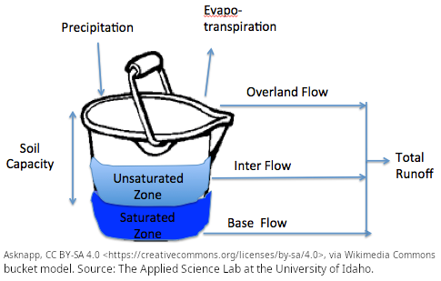
Figure 3. Bucket model. Source: The Applied Science Lab at the University of Idaho.
6. Structure of deterministic models
Deterministic models can be distinguished into two main categories:
- Process based models;
- Empirical models, or black-box models.
A process-based model describes a system by explicitly representing the mechanisms that drive it. It uses mathematical equations based on scientific theory to simulate how components interact over time. The model attempts to replicate real-world processes rather than only fitting observed data. This approach allows researchers to explore scenarios and understand system dynamics. However, such models often require detailed knowledge, in terms of understanding of the underlying processes and description of the system at the microscale.
An empirical model is built by analyzing experimental or observational data to identify relationships between variables. Instead of representing underlying processes, it focuses on empirical relationships in the data. Methods such as regression, machine learning, or statistical fitting are commonly used. These models can provide accurate predictions for known conditions. Their limitation is that they may lack explanatory power about why the system behaves as it does.
Notably, an interesting grey zone exists between process-based models and empirical ones. An example is given by the physics-informed statistical representations. These combine physical knowledge with statistical methods to model complex systems. They incorporate known physical laws, constraints, or equations into statistical modeling frameworks. This helps ensure that predictions remain consistent with established scientific principles. Such models can improve accuracy when data are limited or noisy by guiding learning with physics. They are increasingly used in fields like environmental science, engineering, and climate modeling.
7. An interesting option: machine learning
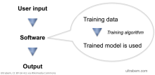
Machine learning models are computational methods that allow computers to learn patterns and relationships from data without being explicitly programmed for every task. They are a central part of the field of Machine Learning, which focuses on developing algorithms that improve their performance through experience.
These models analyze datasets to identify structures, trends, and correlations that can be used for prediction or decision-making. Instead of relying solely on predefined equations, they adapt their internal parameters based on training data. Machine learning models are commonly trained using large datasets to capture complex relationships between input variables and outputs. Once trained, the model can make predictions or classify new, unseen data. There are several main types of machine learning approaches, including supervised learning, unsupervised learning, and reinforcement learning.
In supervised learning, models are trained with labeled examples, where the correct output is already known. In unsupervised learning, the model tries to discover hidden patterns or groupings within unlabeled data. Reinforcement learning focuses on learning through interaction with an environment, using rewards and penalties to guide improvement. Machine learning models can take many forms, such as decision trees, neural networks, and support vector machines. They are widely used in applications like image recognition, recommendation systems, and predictive analytics.
The performance of these models depends on factors such as data quality, model complexity, and training methods. Proper evaluation and validation are important to ensure that models generalize well to new data. As computing power and data availability increase, machine learning models continue to play a growing role in science, technology, and industry.
8. Machine learning: Random Forest
A Random Forest is a machine learning algorithm that can be used for both classification and regression tasks. It is part of the ensemble learning family, where multiple models are combined to improve overall predictive performance. While results are computed by including a random component in order to filter noise in the data and the signal, random forest is considered a deterministic model delivering a point output with no uncertainty assessment in its original formulation.
The algorithm makes classification and regression by following a decision tree, namely, a decision structure that uses a tree-like model of decisions and their possible consequences, including random outcomes, resource costs, and utility. Decision trees are frequently used in operations research to help identify a strategy most likely to reach a goal. They are also a popular tool in machine learning. For an example, see Figure 4. In this case, splits in the tree are in the form of yes/no. In general, splits may be regulated by probabilities, like 30% yes and 70% no and a cost/utility may be associated to given steps of the decision.

Figure 4. Example of a decision tree. By Stefan Lew, based on work of WolfgangW, public domain, via Wikimedia Commons.
To understand how a random forest model works, let's make a simple example where a variable \(Y\) is to be regressed against a single explanatory variable \(X\), to determine the relationship
\(Y=f(X)\)
to be trained (calibrated) by using \(m\) paired observations of \(X\) and \(Y\). The decision tree works by splitting the range of \(X\) in \(n+1\) subranges, where \(n\) is the depth of the tree. Let's suppose that \(n=1\), thus the range of \(X\) is split into two subranges, \(X\leq t\) and \(X \gt t\) where \(t\) is a threshold value to be trained.
Accordingly, the \(Y\) values are divided into two corresponding groups, as any observed \(Y\) values is associated to a corresponding observed value of \(X\). The average value \(\overline{Y_1}\) and \(\overline{Y_2}\) is computed for any of the two groups of \(Y\) values and is stored in what are called the "leaves" of the tree.
The value of \(t\) (the position of the threshold) is determined by minimizing:
\(MSE=\frac{1}{m}\sum_{i=1}^m\left(Y_i−\overline Y_{1,2}\right)^2 \)
therefore minimising the distance between each \(Y\) value and the mean value of \(Y\) in the same group (1 or 2).
In prediction, any input value \(X_{pred} \le t\) is then assigned an output value \(Y_{pred}= \overline{Y_1}\) and any input value \(X_{pred} \gt t\) is then assigned an output value \(Y_{pred}= \overline{Y_2}\).
In general, the depth of the tree may be larger than \(n=1\) therefore splitting in more than 2 groups. The deeper the tree the more accurate the fitting but the larger the chance of overfitting, which implies poor performances in prediction.
We may then decide to further split the decision by adding, for instance, an additional explanatory variable. Then, after splitting \(X\) into subranges, we may again split them according to another decision criteria therefore increasing the nodes of the tree.
Instead of relying on a single decision tree, a Random Forest constructs a large number of decision trees during the training phase. Each tree is built using a different random subset of the training data, a process known as bootstrapping or bagging. Additionally, at each split in a tree, the algorithm considers only a random subset of the available explaining variables to determine the best split.
This randomness introduces diversity among the trees and helps reduce correlation between them. As a result, the model becomes more robust and less prone to overfitting compared to a single decision tree. When predictions are made, each tree in the forest produces its own output independently. For classification problems, the final prediction is determined by majority voting among all trees. For regression problems, the predictions from all trees are averaged to obtain the final result.
Random Forest models are known for their strong predictive accuracy and their ability to handle large datasets with many features. They are also relatively robust to noise and missing data in the training set. Another advantage of Random Forests is that they can estimate feature importance, allowing researchers to understand which variables contribute most to the model’s predictions. Due to these strengths, Random Forests are widely applied in fields such as healthcare, finance, environmental science, and bioinformatics. Overall, the algorithm provides a powerful and flexible approach for building reliable predictive models while maintaining good generalization performance on unseen data.
In the context of environmental sciences, Random Forest models are frequently used for predicting unknown variables depending on known inputs. Another example of a decision tree is given by Figure 5.
In summary Random Forest:
- Reduces overfitting: averaging many trees lowers variance;
- Captures nonlinearity: trees model complex relationships between input and output variables.
- It is Robust: less sensitive to noise and outliers than a single tree. A single decision tree can be unstable because it relies on only one opinion. The random forest is analogous to a committee of noisy but diverse experts, from which we take the average consensus as final prediction.

Figure 5. Schematic of a random forest algorithm. By TseKiChun, CC BY-SA 4.0, via Wikimedia Commons.
8.1 A simple example through a Python code
Try the code below to see how random forest works.
import matplotlib.pyplot as plt
from sklearn.ensemble import RandomForestRegressor
#Generate data through a sinusoidal function plus noise
np.random.seed(0)
X = np.sort(5 * np.random.rand(100, 1), axis=0)
y = np.sin(X).ravel() + 0.3 * np.random.randn(100)
# 2. Train model
rf = RandomForestRegressor(n_estimators=50)
rf.fit(X, y)
# 3. Predict
X_test = np.linspace(0, 5, 500).reshape(-1, 1)
y_pred = rf.predict(X_test)
# 4. Plot
plt.scatter(X, y)
plt.plot(X_test, y_pred)
plt.title("Random Forest Regression")
plt.xlabel("X")
plt.ylabel("Y")
plt.show()
Try with the above code the following:
- n_estimators=1 (a single tree, namely, a step function);
- n_estimators=200 (a smoother curve);
- max_depth=2 (very rough approximation);
- min_samples_leaf=10 (smoother, less noisy).
8.2 A simple example through a R code
Try also the code below which again simulates and then fits a sinusoidal function. Note: here we include more than one explanatory variable, by consider also previous data points as input data. This is useful in time series modelling.
install.packages("dplyr")
library(randomForest)
library(dplyr)
time = 1:100
value = sin(time/5) + rnorm(100, 0, 0.2)
data = data.frame(time, value)
plot(data,type="l")
#With the instruction below we lag the data to build more explanatory variables
#with the lagged data
data = data %>%
mutate(
lag1 = lag(value, 1),
lag2 = lag(value, 2),
lag3 = lag(value, 3)
)
data = na.omit(data)
train_size = floor(0.8 * nrow(data))
train = data[1:train_size, ]
test = data[(train_size+1):nrow(data),]
model = randomForest(
value ~ lag1 + lag2 + lag3,
data = train, ntree = 200
)
predictions = predict(model, newdata = test)
rmse = sqrt(mean((predictions - test$value)^2))
print(rmse)
plot(test$value, type = "l", col = "blue", lwd = 2)
lines(predictions, col = "red", lwd = 2)
legend("topright",
legend = c("Actual", "Predicted"),
col = c("blue", "red"),
lty = 1)
importance(model)
varImpPlot(model)
9. Machine learning: Neural Networks
A neural network (NN), also known as artificial neural network (ANN), is a deterministic input-output relationship inspired by the shape and workflow of biological neural networks.
A neural network is made up by connected nodes called artificial neurons. These are connected by edges. Each artificial neuron receives signals from other connected neurons, then elaborates them and sends the elaborated signal to other connected neurons. The signal is a real number, and the output of each neuron is given by a non-linear function of its inputs: the activation function. The signal at each connection is weighted through a weight, which is calibrated during the learning process. See figure 6.

Figure 6. Scheme of an artificial neural network
Typically, neurons are displaced into layers. A network may count an arbitrary number of layers, which perform different transformations on their inputs. Signals travel from the input layer (the first layer) to the output layer (the last layer), possibly passing through intermediate layers which are called hidden layers.
Advances in computing power and the availability of large datasets further stimulated the evolution and application of neural networks in the early 21st century. The elaboration of sophisticated structures like convolutional neural networks (CNNs) significantly improved performance in computer vision tasks, while recurrent neural networks (RNNs) enabled modeling of sequential data such as time series. More recently, attention has been given to structures allowing to model long-range dependencies in data, like the LSTM network described below.
9.1 LSTM networks
A Long Short-Term Memory (LSTM) network is a type of recurrent neural network designed to model sequential data while overcoming one of the main limitations of traditional recurrent models, namely, models that are designed to work with sequences of data by remembering past information: their difficulty in learning long-term dependencies.
In many real-world problems such as language modeling, speech recognition, or time series forecasting, the current output depends not only on recent inputs but also on information that may have occurred many time steps earlier, thus originating long term persistence (or long term/long range dependence), originating the so-called Hurst effect. Standard recurrent neural networks struggle in these settings because, during training, the improvement of results obtained by changing a given weight may become negligible, in particular for weights that are located far from the output layer.
In fact, neural network are typically trained through backpropagation. Backpropagation (short for backward propagation of errors) is the algorithm that neural networks use to learn from their mistakes. In fact, training a neural network happens in two phases: there is the forward pass first, where the input goes through the network thus produces an output. Then, there is the backward pass, or backpropagation, where the model compares output to the correct answer, computes the error and sends it backward to update the weights. In essence, the network makes a prediction, checks how wrong it was and then it finds which weights caused the error and how these should be adjusted.
A challenge for ANN training is given by the gradients used to update the model parameters tending to either vanish or explode as they are propagated backward through time. It is the vanishing gradient problem. The weights located close to the output layer explain most of the error and therefore little information remains to update weights located at greater distance. This makes it hard for the network to retain useful information over long sequences. LSTMs address this issue by introducing a more structured and controlled way of storing and updating information.
At the core of an LSTM is a memory cell (or unit), which can be thought of as a running summary of the past. The memory cell is characterised by a cell state, \(C_t\) and a hidden state \(h_t\). The cell state is a long-term storage of the past memory, while the hidden state is what is passed to the output depending on cell state and network structure. In other words, the hidden state in an LSTM is the current, usable representation of past information, passed forward through the sequence to guide future predictions.
Cell state and hidden state are updated at every time step through a set of carefully designed components called gates. These gates regulate the flow of information into and out of the memory, allowing the network to decide what to keep, what to discard, and what to output. Each gate is implemented as a small neural network layer that produces values between zero and one, effectively acting as a soft switch.
The first of these components is the forget gate, whose role is to determine which parts of the existing memory are no longer relevant. By examining both the current input and the previous hidden state, the forget gate assigns a weight to each of them, where values close to zero correspond to information that should be discarded and values close to one correspond to information that should be retained. This selective forgetting is crucial, as it prevents the memory from becoming cluttered with outdated or irrelevant information.
The second component is the input gate, which controls how much new information should be written into the memory. This process involves two steps: first, the network generates a candidate representation of new information based on the current input and previous hidden state; second, the input gate determines how strongly this candidate should influence the memory. The candidate values are typically passed through a hyperbolic tangent function, which constrains them within a bounded range and allows both positive and negative contributions. The combination of the input gate and the candidate memory enables the network to incorporate new, relevant signals while ignoring noise.
Once the forget and input operations have been applied, the memory cell is updated by combining the retained past information with the selected new content, through the so called candidate gate (or cell candidate). This additive update mechanism is one of the key features that allows LSTMs to mitigate the vanishing gradient problem, as it provides a more stable path for gradient flow during training. The updated memory can therefore carry meaningful information across many time steps.
The final component is the output gate, which determines what part of the internal memory should be exposed as the hidden state. The hidden state serves both as the output of the LSTM at the current time step and as an input to the next time step. By filtering the memory through the output gate, the network can focus on the most relevant aspects of its internal state for the task at hand.
Let's look at the structure of a LSTM in detail:
- Forget Gate: decides what information to discard from memory, depending on previous hidden state \(h_{t-1}\) and current input \(x_t\). The response from the forget gate is a value between 0 (forget everything) and 1 (keep everything), that is computed through a linear transformation of \(h_{t-1}\) and \(x_t\) through the weights, followed by a sigmoid function to rescale in the range [0,1]. The result is the value of the forget gate \(f_{t}\).
- Input Gate: decides what new information to store in the current hidden state \(h_{t}\), depending on previous hidden state \(h_{t-1}\) and current input \(x_t\). In the input gate, computations are rescaled through the sigmoid function \(\sigma\), rescaling results in the range [0,1]. The result is the value of the input gate \(i_{t}\).
- Computation of candidate new information \(\tilde C_{t}\), depending on previous hidden state \(h_{t-1}\) and current input \(x_t\). The results is rescaled by the hyperbolic tangent function \(\tanh\), rescaling values in the range [-1,1] therefore allowing to store negative values when memory is to be forgotten.
- Update of the cell state, depending on \(f_{t}\), \(i_{t}\), \(C_{t-1}\), and \(\tilde C_{t}\).
- Output Gate: decides what to output, by computing \(o_{t}\) depending on \(h_{t-1}\) and \(x_{t}\).
- Update of the hidden state, depending on \(o_{t}\) and \(C_{t}\).
- Obtain the final result through an output layer called "dense layer" which maps the hidden state into the scale of the variable to be predicted.
Therefore, the step-by-step flow at each time step is as follows:
- Forget old info, by removing irrelevant parts from the cell state;
- Add new information, by update memory with useful new data;
- Compute output, by producing the hidden state for next step and rescale it in the scale of the prediction.
The above computation is done by a "unit" (or cell) of the LSTM network (Figure 7), which operates a linear transformation and a rescaling in each gate. A LSTM may include several units. They all process the same information but through optimization they account for different patterns in the data.
See the scheme in Figure 7 and look at the numerical example below to better understand the workflow in the figure.
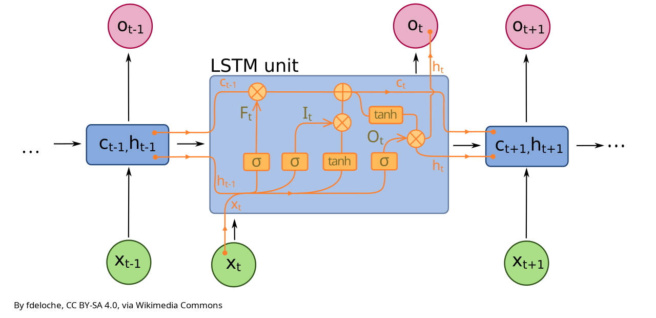
Figure 7. Scheme of a unit of a LSTM network.
9.2 LSTM networks: numerical examples
Let’s go step by step through a trivial numerical example (with simple numbers) of a single unit LSTM cell at one time step where:
- Input is \(x_t = 1.0\);
- Previous hidden state is \(h_{t-1} = 0.5\);
- Previous cell state is \(C_{t-1} = 0.2\).
- Weights of the forget gate are \(W_f = [0.7, 0.3]\) and bias of the forget gate is \(b_f=0\);
- Weights of the input gate are \(W_i = [0.6, 0.4]\) and bias of the input gate is \(b_i=0\);
- Weights for the computation of candidate representation of new information (candidate gate): \(W_c = [0.5, 0.5]\) and related bias \(b_c=0\);
- Weights for the computation of output (output gate): \(W_o = [0.4, 0.6]\) and related bias \(b_o=0\);
Then the computation is articulated along the following steps:
- Forget Gate: \(f_t = \sigma(W_f \cdot [h_{t-1}, x_t] + b_f) = \sigma(0.7 \cdot 0.5 + 0.3 \cdot 1.0) = \sigma(0.35 + 0.3) = 0.66\), namely, keep 66% of old memory;
- Input Gate: \(i_t = \sigma(W_i \cdot [h_{t-1}, x_t] + b_i) = \sigma(0.6 \cdot 0.5 + 0.4 \cdot 1.0) = \sigma(0.3 + 0.4) = 0.67\);
- Candidate representation of new information: \(\tilde{C_t} = \tanh(W_c \cdot [h_{t-1}, x_t]+b_c = \tanh(0.5 \cdot 0.5 + 0.5 \cdot 1.0) = \tanh(0.75) \approx 0.64\);
- Updating of Cell State: \(C_t = f_t \cdot C_{t-1} + i_t \cdot \tilde{C}_t = 0.66 \cdot 0.2 + 0.67 \cdot 0.64 \approx 0.561\);
- Computation of output gate: \(o_t = \sigma(W_o \cdot [h_{t-1}, x_t] = \sigma(0.4 \cdot 0.5 + 0.6 \cdot 1.0 = 0.2 + 0.6) \approx 0.69\);
- Computation of new hidden State, which for simplicity we assume it is our final result (we skip mapping along the range of the predicted variable): \(h_t = o_t \cdot \tanh(C_t) \approx 0.35\).
The the final results are:
- Output at time \(t = 0.69\);
- Cell state \(C_t ≈ 0.56\);
- Final result (hidden state) \( h_t ≈ 0.35\).
Basically the forget gate kept most of the old memory, the input gate added new useful information, the cell state updated the memory and the output gate filtered the whole information to compute the prediction.
Let’s walk through a multi-step sequence to better clarify evolution over time. We will use the same LSTM, same weights and biases of the previous example and we again skip the mapping through the dense layer.
Inputs sequence: \( x = [1.0,; 0.5,; -1.0]\); initial states: \(h_0 = 0, C_0 = 0\); same weights as before: forget: \(W_f = [0.7, 0.3]\); input: \(W_i = [0.6, 0.4]\); candidate: \(W_c = [0.5, 0.5]\); output: \(W_o = [0.4, 0.6]\).
Time Step 1:
\( x_1 = 1.0\);
Input: \([h_0, x_1] = [0, 1]\);
Forget: \( f_1 = \sigma(0.3) \approx 0.57\);
Input: \( i_1 = \sigma(0.4) \approx 0.60 \);
Candidate: \(\tilde{C}_1 = \tanh(0.5) \approx 0.46\);
Cell state: \(C_1 = 0.57 \cdot 0 + 0.60 \cdot 0.46 \approx 0.28\);
Output: \(o_1 = \sigma(0.6) \approx 0.65 \);
Hidden (result): \(h_1 = 0.65 \cdot \tanh(0.28) \approx 0.65 \cdot 0.27 \approx 0.18\).
Time Step 2:
\(x_2 = 0.5\);
Input: \([h_1, x_2] = [0.18, 0.5]\);
Forget: \(f_2 = \sigma(0.7·0.18 + 0.3·0.5) = \sigma(0.276) \approx 0.57\);
Input: \(i_2 = \sigma(0.6·0.18 + 0.4·0.5) = \sigma(0.308) \approx 0.58 \);
Candidate: \(\tilde{C}_2 = \tanh(0.34) \approx 0.33\);
Cell state: \(C_2 = 0.57·0.28 + 0.58·0.33 \approx 0.16 + 0.19 = 0.35\);
Output: \(o_2 = \sigma(0.372) \approx 0.59\);
Hidden (result): \( h_2 = 0.59 \cdot \tanh(0.35) \approx 0.59 \cdot 0.34 \approx 0.20\);
Time Step 3:
\( x_3 = -1.0 )\);
Input: \([h_2, x_3] = [0.20, -1.0]\);
Forget: \(f_3 = \sigma(0.14 - 0.3) = \sigma(-0.16) \approx 0.46\);
Input: \( i_3 = \sigma(0.12 - 0.4) = \sigma(-0.28) \approx 0.43\);
Candidate: \(\tilde{C}_3 = \tanh(-0.4) \approx -0.38\);
Cell state: \(C_3 = 0.46·0.35 + 0.43·(-0.38) \approx 0.16 - 0.16 \approx 0.00\);
Output: \(o_3 = \sigma(-0.52) \approx 0.37\)
Hidden (result): \( h_3 = 0.37 \cdot \tanh(0.00) = 0\).
Summary of the evolution:
| Step | Input | Cell State \(C_t\) | Output \(0_t\) | Hidden \(h_t\) |
|---|---|---|---|---|
| 1 | 1.0 | 0.28 | 0.65 | 0.18 |
| 2 | 0.5 | 0.35 | 0.59 | 0.20 |
| 3 | -1.0 | ~0.00 | 0.37 | 0.00 |
During the steps 1–2 there is positive input which builds memory up and the LSTM keeps account for past signal. At step 3 there is negative input, the candidate becomes negative so that the forget gate weakens old memory. Negative signal from the input implies that memory gets erased, so that The LSTM deletes what is considered to be no longer relevant.
Now let's refer to another example to make 1 step prediction by using LSTM for variable \(y_{t+1}\) depending on \(y_t\), \(y_{t-1}\) and an exogenous variable \(x_t\). we assume 1 unit only for the LSTM and assume all weights and biases are known.
The input vector has size 3 and is:
\(z_t = [y_t, y_{t-1}, x_t]\);
By recalling what we wrote above, the LSTM equations are:
\(f_t = \sigma(W_f z_t + U_f h_{t-1} + b_f)\);
\(i_t = \sigma(W_i z_t + U_i h_{t-1} + b_i)\);
\(\tilde{c}*t = \tanh(W_c z_t + U_c h*{t-1} + b_c)\);
\(c_t = f_t c_{t-1} + i_t \tilde{c}*t\);
\(o_t = \sigma(W_o z_t + U_o h*{t-1} + b_o)\);
\(h_t = o_t \tanh(c_t)\);
and then, for the final output layer (the dense layer):
\(y_{t+1} = W_y h_t + b_y\).
Note that now we apply the dense layer to compute the final result.
We can write the code by first writing a function to make the prediction. Then we run it through a second code where weights are defined. The code for the function follows here below.
sigmoid = function(x) {
1 / (1 + exp(-x))
}
# Function applying LSTM
lstm_one_step = function(y_t, y_t_minus_1, x_t,
h_prev, c_prev,
params) {
# Input vector (length = 3)
z_t = c(y_t, y_t_minus_1, x_t)
# Extract parameters
#Forget gate
W_f = params$W_f # (1x3)
U_f = params$U_f # scalar
b_f = params$b_f
#Input gate
W_i = params$W_i
U_i = params$U_i
b_i = params$b_i
#Candidate state gate
W_c = params$W_c
U_c = params$U_c
b_c = params$b_c
#Outout gate
W_o = params$W_o
U_o = params$U_o
b_o = params$b_o
#Dense layer
W_y = params$W_y
b_y = params$b_y
# Gates
f_t = sigmoid(sum(W_f * z_t) + U_f * h_prev + b_f)
i_t = sigmoid(sum(W_i * z_t) + U_i * h_prev + b_i)
c_tilde = tanh(sum(W_c * z_t) + U_c * h_prev + b_c)
# Cell state
c_t = f_t * c_prev + i_t * c_tilde
# Output gate
o_t = sigmoid(sum(W_o * z_t) + U_o * h_prev + b_o)
# Hidden state
h_t = o_t * tanh(c_t)
# Final prediction (through the dense layer)
y_next = W_y * h_t + b_y
return(list(
y_next = y_next,
h_t = h_t,
c_t = c_t
))
}
Now let's write the code to run the above function.
params = list(
W_f = c(0.2, -0.1, 0.05),
U_f = 0.1,
b_f = 0.0,
W_i = c(-0.3, 0.2, 0.1),
U_i = 0.05,
b_i = 0.0,
W_c = c(0.4, 0.1, -0.2),
U_c = 0.1,
b_c = 0.0,
W_o = c(0.1, -0.2, 0.3),
U_o = 0.05,
b_o = 0.0,
W_y = 1.0,
b_y = 0.0
)
# Initial states
h_prev = 0
c_prev = 0
# Inputs
y_t = 1.2
y_t_minus_1 = 1.0
x_t = 0.5
# Run one-step prediction
res = lstm_one_step(y_t, y_t_minus_1, x_t,
h_prev, c_prev,
params)
print(res$y_next)
Training an LSTM involves learning the weights and biases associated with all these gates and transformations. This is typically done using backpropagation through time, an extension of the standard gradient descent algorithm to sequential data. Through this process, the network gradually learns how to manage its memory in a task-specific way, identifying patterns in the data that require long-term retention and those that can be safely ignored.
9.2 LSTM networks: two example codes in R
Let's now try to run a toy LSTM in R to better understand the workflow. We start with a simple LSTM where we want to predict a variable Y at each time step depending on current and past 4 values of a single explanatory variable X.
install.packages("keras3")
library(keras3)
# Prepare data by generating a simple linear dependence between X and Y
n = 100
x = rnorm(n)
y = 0.8*x+rnorm(n,sd=0.1)
# Combine into features
data = cbind(y, x)
# Create sequences of current time and past four X values to explain current time Y
# Note: keras input data is a matrix with dimension (samples, timesteps, features)
# Samples is the number of samples of 5 values used to train the model
# Timesteps is the number of time steps of X to explain Y (5)
# Features is the number of exogenous variables (1 in this case)
X = array(0, dim=c(96,5,1))
for (i in 1:(nrow(data) - 4))
X[i,,] = data[i:(i+4),2]
# Now we build the vector of variable to predict (future Ys)
Y=y[5:100]
# Build LSTM model
model = keras_model_sequential() %>%
layer_lstm(units = 20, input_shape = c(5, 1)) %>%
#Note the number of units, which is quite large
layer_dense(units = 1)
# Specifies the size of the output - We predict one number only
model %>% compile(
loss = "mse",
optimizer = "adam"
)
# Train
model %>% fit(X, Y, epochs = 20, batch_size = 10)
# Prediction
pred = model %>% predict(X)
An interesting question: how many parameters (weights and biases) does the above LSTM counts? To answer to the question, consider that the networks counts 20 "units": as we mentioned above, a unit (see Figure 7) is the elementary component of the LSTM network including 4 gates: forget gate, input gate, candidate gate, output gate. Note that in the above network the hidden state is a vector with length 20, as we have 20 units and each unit has a hidden state. Therefore, each hidden state weight is actually a vector with length 20. Therefore, for each unit we count 4 weights for the input (one each gate), 20 weights for the previous state (five each gate), 4 weights for the bias (one each gate). The total is 28 weights each unit; we have 20 units, therefore the total is 560.
At this point, we need to add the weights of the dense layer: it is a final layers that combines the 20 outputs from the 20 units into a single number, through a linear combination of the 20 outputs plus a bias.
To conclude: the above LSTM includes 581 weights.
For comparison, let's try a second code where the current value of Y is predicted depending on the current value of X and the past value of Y.
n = 100
x = rnorm(n)
y = 0.8*x+rnorm(n,sd=0.1)
# Combine into features
data = cbind(y, x)
# Create sequences of current time and past four X values to explain current time Y
# Note: keras input data is a matrix with dimension (samples, timesteps, features)
# Samples is the number of samples of 5 values used to train the model
# Timesteps is the number of time steps of X to explain Y (5)
# Features is the number of exogenous variables (1 in this case)
X = array(0, dim=c(99,1,2))
for (i in 2:(nrow(data)))
{
X[i-1,1,1] = data[i,2]
X[i-1,1,2] = data[i-1,1]
}
# Now we build the vector of variable to predict (future Ys)
Y=y[2:100]
# Build LSTM model
model = keras_model_sequential() %>%
layer_lstm(units = 20, input_shape = c(1, 2)) %>%
layer_dense(units = 1)
# Specifies the size of the output - We predict one number only
model %>% compile(
loss = "mse",
optimizer = "adam"
)
# Train
model %>% fit(X, Y, epochs = 20, batch_size = 10)
# Prediction
pred = model %>% predict(X)
Conclusion
This lecture hopefully offered to you a panorama of different solutions to obtain a deterministic estimation of environmental forcing under climate change. Beware that many other examples could be provided. For instance, in the domain of linear models ARIMA modelling has been widely used. These are stochastic processes providing a deterministic prediction along with uncertainty assessment. Although they are not strictly speaking deterministic models, very often they have been applied by discarding the random component for obtaining a deterministic linear prediction, also basing on exogenous inputs.
The set of deterministic models is very large and offers a myriad of interesting solutions.
Last revised on May 20, 2026
- 248 views