


[This lecture was partially created with the support of Artificial Intelligence tools (ChatGPT)]
Introduction
Extreme Value Theory (EVT) is a branch of statistics dedicated to understanding the behavior of rare and extreme events rather than typical or average conditions. Often these events have never yet been observed, and their probabilities must therefore be estimated by extrapolation of models fitted to available data. Because data concerning the event of interest may be very limited, efficient methods of inference play an important role.
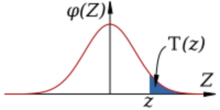
Therefore, unlike classical statistics, which focuses on the whole range of the considered variable, EVT concentrates on the most unfrequent realisations, that is on what is called the "tails" of probability distributions. With the term "tail" we identify the portions of the probability density functions corresponding to very low probability of exceedance and not exceedance (see Figure 1).
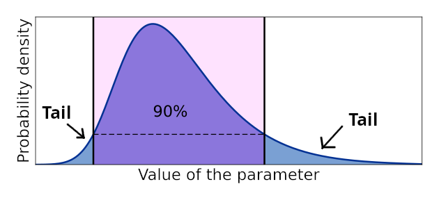
Figure 1. Tails of the probability density function. Modified after Justinkunimune, CC0, via Wikimedia Commons.
This tail-focused perspective is crucial when the most severe events dominate risk and potential damage. Examples include extreme wind speeds, intense rainfall, large ocean waves, floods, and heatwaves. In many natural and engineered systems, failure is driven by extremes rather than everyday loads.
EVT is therefore widely used in engineering, climate science, hydrology, finance, and risk analysis. Designing structures or systems based only on average conditions can lead to unsafe or non-resilient outcomes. EVT provides tools to estimate the magnitude and likelihood of events that may occur once in decades or centuries. These estimates form the basis of return periods, such as the “100-year event,” commonly used in design standards. By focusing on extremes, EVT supports risk-informed decision-making under uncertainty.
A key contribution of EVT is its theoretical insight into how extreme events behave statistically. It shows that the distribution of extremes follows specific limiting forms, regardless of the underlying data distribution. This universality makes EVT especially valuable when observations are scarce or highly variable. However, applying EVT requires careful statistical judgment and understanding of assumptions. As a result, EVT is both a powerful and a subtle tool for analyzing rare but impactful phenomena.
We will get into extreme value theory with a "learning by doing" approach. Learning by doing is a way of learning through direct experience and action, using data to identify a problem and learn how the theory helps in solving it, instead of following the classical approach that moves from theory to application. Making mistakes is part of the process and helps deepen understanding, by connecting the theory to real-world problems. Our approach will not follow a rigorous and comprehensive treatment of any detail of the theory. It will rather focus on what we need to reliably estimate loads in the presence of climate change.
The basis of extreme value theory
We already learned that EVT is a branch of statistics. In turn, statistics is the discipline that concerns the collection, organization, analysis, interpretation, and presentation of data. In applying statistics to a scientific, industrial, or social problem, it is conventional to begin with a statistical population, namely, a set of similar items or events which is of interest for some question. To make these events tractable with an analytic process, events themselves are usually associated to numbers, therefore obtaining realisations from a random variable, that is, a formalization of a quantity or object which depends on random events.
Then, an objectives of statistics is to identify models to explain patterns. Several possible interpretations of patterns (models) can be used to get to target. The most classical approach is to use probability theory to identify a model and test it. Quoting from Wikipedia:
Although there are several different probability interpretations, probability theory treats the concept in a rigorous mathematical manner by expressing it through a set of axioms. Typically these axioms formalise probability in terms of a probability space, which assigns a measure taking values between 0 and 1, termed the probability measure, to a set of outcomes called the sample space. Any specified subset of the sample space is called an event.
Alternatives to probability include:
Fuzzy logic – handles uncertainty using degrees of truth (e.g., “somewhat likely”) instead of exact probabilities.
Possibility theory – models what is plausible rather than how likely something is.
Evidence theory (Dempster–Shafer theory) – represents uncertainty using belief and plausibility, not fixed probabilities.
Deterministic models – assume no uncertainty and produce exact outcomes based on inputs.
Here, we will focus on probability and deterministic models (in another lecture).
In statistics, extreme values are uncommon observations that appear well away from the typical range. Rather than concentrating on central measures such as the mean or median, EVT specifically studies these rare outcomes. For example, while average rainfall describes normal weather conditions, EVT focuses on unusual events like extreme storms or droughts. By analyzing extremes, EVT helps estimate the likelihood and risk of rare but high-impact events.
A synthetic time series
Let us start our treatment of EVT by generating a synthetic time series with the following R code:
A=exp(A)
thus obtaining the series depicted in figure 2 with density given in figure 3.
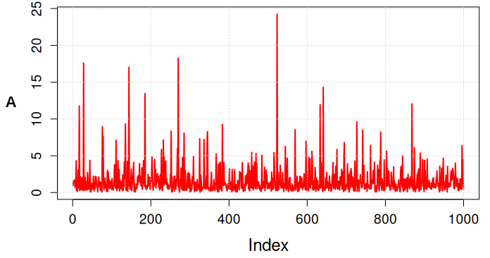
Figure 2. Series generated with the R code.
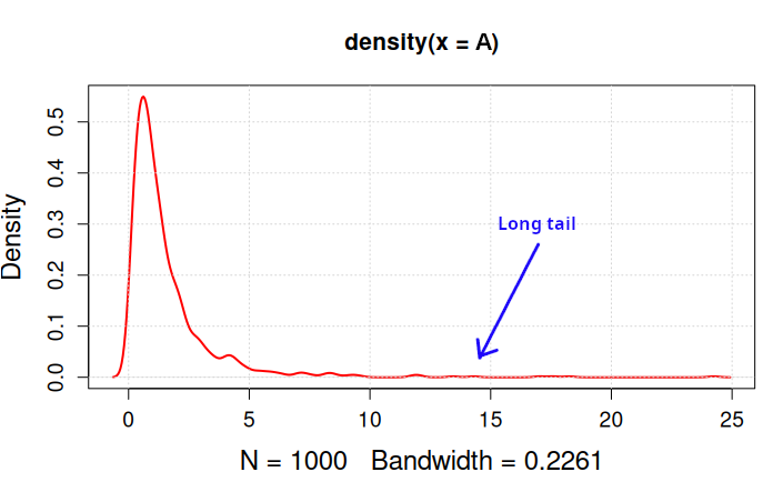
Figure 3. Density of the series generated with the R code.
The density clearly shows the long tail of the series, that has been generated according to the lognormal distribution (we obtain data following the normal distribution by taking the natural logarithm of the series). Note that we generated the data by taking the exponential of a random generation from a Gaussian distribution with mean 0 and standard deviation 1.
The question now is: had we obtained the data from observing a given event (like for instance wave height), how can we estimate the probability of very rare outcomes?
Let's make it more challenging: what is the probability of getting an outcome of A equal to, say, W=max(A)+5? Of course we cannot exclude that such a value occurs. We understand it must have very low probability, but what is the value of the probability of not exceedance of W?
Focusing on the tail
Of course, there is the obvious solution of fitting a probability distribution to the whole data set and then extrapolating the estimated density beyond the observed data range. For the above case of the synthetic series it may indeed work, because the data are independent, identically distributed (they were generated by the lognormal distribution), and the sample size is satisfactorily large. Get familiar with the status of data being "independent and identically distributed" because this is a crucial assumption when estimating probabilities.
If data are not independent, a possible solution is to make a selection from the collection of events, piking up large ones that are independent each other. If data are not identically distributed, the solution is to focus on the tail, once again by picking up large events.
There are two strategies that are largely applied in order to focus on large and independent outcomes. The first strategy is called "block maxima" approach. Data are divided in windows (blocks) of equal size and the maximum is picked up from each window (Figure 4). Blocks need to be sufficiently large to make sure that the selected events are indeed independent. An approach that is frequently applied to time series is the "annual maxima" method, where the blocks have length of one year (see for instance here; see also Figure 4).
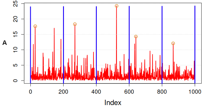
Figure 4. Block maxima approach. Yellow circles identify the values that are picked up.
The block maxima approach is particularly useful for analyzing annual maxima, like yearly peak rainfall. On the other hand, it has the limitation that it uses only block maxima, discarding other extreme values within the block, which may lead to loss of information.
A second strategy is to select data point that exceed a given threshold: this is the "peak over threshold method" (POT, see here and here; see also Figure 5).
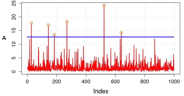
Figure 5. Peak over threshold approach. Yellow circles identify the values that are picked up.
The POT method utilises more data by considering all exceedances, offering a more detailed view of extremes. The most important limitation is that it requires careful selection of the threshold, as too low or high a threshold can skew results. In particular, a low threshold may lead to selecting events that are not independent.
Let's look at the above two approaches in detail.
Block maxima
A compelling question when analysing extreme values is what distribution to use. We should of course look for the most appropriate distribution and therefore we need to look at the theory: what is the behaviour of block maxima? Does it exist a distribution that describes them optimally? Remember that we often deal with limited sample sizes. The convergence of data to a distribution may be asymptotic, meaning that different distributions may suit the data optimally for limited and large sample sizes.
Asymptotic convergence is studied by asymptotic analysis. The following example of asymptotic behaviour is given by Wikipedia here:
As an illustration, suppose that we are interested in the properties of a function f (n) as n becomes very large. If f(n) = n2 + 3n, then as n becomes very large, the term 3n becomes insignificant compared to n2. The function f(n) is said to be "asymptotically equivalent to n2, as n → ∞". This is often written symbolically as f (n) ~ n2, which is read as "f(n) is asymptotic to n2."
Another example of asymptotic convergence is given by the Central Limit Theorem: if one adds up lots of random variables → the sum tends to a normal distribution.
So, what happens if one selects the maxima from a large number of large blocks? The answer is given by the Fisher–Tippett-Gnedenko Theorem (1928), which is the extremes version of the Central Limit Theorem:
Take the maximum (or minimum) of lots of random variables → after proper rescaling, it converges to one of only three possible distributions, no matter what the original distribution was.
So:
- Sums → Normal;
- Maxima → One of three “extreme value” distributions, which we introduce now.
Let \(X_1\), \(X_2\), ... \(X_n\) be independent and identically distributed (IID, note, this assumption is crucial) random variables with some unknown distribution \(F\). They could be, for instance, observations of daily rainfall for one year, so \(n=365\). Define the maximum:
\(M_n\)=max\( (X_1, X_2,...,X_n)\).
Then, for the formula of joint probability:
\(P(M_n \le x) = P(X_1 \le x,\dots,X_n \le x)\).
By taking into account independence:
\(P(M_n \le x) = F(x)^n\).
The above equation is the basis of extreme value theory.
Let's make an exercise in Python. We require the preliminary installation of libraries. The instructions below provide library installation guidelines for the Linux Environment (tested on Ubuntu 24.04).
Exercise - Installing Python and pip
Let's check if Python and pip are installed. Open a Linux terminal and check:
pip3 --version
If they are not found, install with
sudo apt install python3
sudo apt install python3-pip
Then, install the packages that are requested (the packeges imported into the codes may need to be installed). We provide an example by installing the packages requests and pyextremes that we need to run other exercises later on.
pip install requests
If pip install does not work, you may try by creating a virtual environment:
source venv/bin/activate
pip install pyextremes
pip install requests
If you get an error message like:
The virtual environment was not created successfully because ensurepip is not
available. On Debian/Ubuntu systems, you need to install the python3-venv
package using the following command.
apt install python3.12-venv
follow the instructions and install python3-venv as suggested and repeat the code above.
Pyextremes is a Python library aimed at performing univariate Extreme Value Analysis (EVA). It provides tools necessary to perform a wide range of tasks required to perform extreme value analysis.
Now, let's run a first exercise, by launching the following code in a Python console that you can start in Ubuntu by simply running:
The code to run is:
import numpy as np
import seaborn as sns
import pandas as pd
import matplotlib.pyplot as plt
# Empirical CDF of maxima - from standard normal.
X = pd.DataFrame([np.random.normal(size=10).max() for _ in range(1000)])
sns.ecdfplot(X)
plt.show()
Now let's plot the known CDF:
# CDF of maxima - from standard normal cdf.
x = np.linspace(0, 3.5, 100)
cdf_x = 1/2*(1 + erf(x/math.sqrt(2)))
cdf_max_of_10 = np.power(cdf_x, 10)
sns.lineplot(data=pd.DataFrame({'x': x,
'$F(M_{10})$': cdf_max_of_10}),
x='x',
y='$F(M_{10})$')
plt.show()
For large \(n\), however, we experience a problem: if \(F(x)\le 1\) then \(F(x)^n → 0\) as \(n→∞\). If \(F(x)=1\) then \(F(x)^n=1\) and \(M_n→x_F\) where \(x_F\) is the upper bound of the distribution (which may be infinity).
To solve the problem we normalise the maxima with the relationship:
\( \frac{Mn−b_n}{a_n}\)
where \(a_n>0\) and \(b_n\) are constants. For the rescaled data, \(P\left(\frac{M_n−b_n}{a_n}≤z\right)=F(a_n z+b_n)^n\) which converges to a non-degenerate limit \(G(z)\), where \(z\) is the rescaled variable.
The Fisher–Tippett–Gnedenko theorem (1928) states that:
If there exist \(a_n>0\) and \(b_n\) such that
\(\frac{M_n - b_n}{a_n} \xrightarrow{d} G\)
for some non-degenerate distribution \(G\) then \(G\) must belong to one of exactly three families:
- Gumbel (Type I, light-tailed distributions), with CDF:
\( G(z) = \exp\left(-e^{-z}\right) \)
- Fréchet (Type II, Heavy-tailed distributions), with CDF:
\( G(z)=\begin{cases} 0, & z \le 0 \\ \exp(-z^{-\alpha}), & z > 0 \end{cases} \quad \alpha > 0 \)
- Weibull (Type III, bounded distributions), with CDF:
\( G(z)=\begin{cases} \exp\left(-(-z)^\alpha\right), & z \le 0 \\ 1, & z > 0 \end{cases} \quad \alpha > 0 \)
Note that Gumbel counts 2 parameters while Frechet and Weibull count 3 parameters. It can be proved that the Gumbel family arises (asymptotically) when the random variable \(X\) is:
- Exponential;
- Normal;
- Lognormal;
- Gamma.
In other words, the maxima of samples from the normal distribution follow a Gumbel distribution (see exercise below).
Typical examples are:
- Maximum daily temperature;
- Maximum rainfall (moderate extremes).
The Frechet family arises (asymptotically) when the random variable \(X\) is:
- Pareto;
- Cauchy;
- Student-t (low degrees of freedom).
Typical examples are:
- Financial crashes;
- Insurance losses.
The Weibull family arises (asymptotically) when the random variable \(X\) is:
- Uniform;
- Beta (bounded support);
- Any distribution with a hard upper limit.
Typical examples are:
- Maximum strength of a material;
- Physical limits with strict caps.
One-line summary of Fisher–Tippett–Gnedenko Theorem (1928):
If the maximum of many i.i.d. random variables converges (after scaling), its limit must be Gumbel, Fréchet, or Weibull—nothing else is possible.
These three families of distributions can be grouped together under the big family of the Generalised Extreme Value (GEV) distribution. A random variable \(X\) has a GEV distribution with location \(\mu \in \mathbb{R}\), scale \(\sigma > 0\), and shape \(\xi \in \mathbb{R}\) if its cumulative distribution function (CDF) is (note: \(\mu\) and \(\sigma\) are not the mean and standard deviation of the distribution):
\(G(x) =
\begin{cases}
\exp \left\{ -\left[ 1 + \xi \left( \dfrac{x-\mu}{\sigma}\right)\right]^{-1/\xi}\right\},
& \text{if } 1 + \xi \left( \dfrac{x-\mu}{\sigma}\right) > 0,\ \xi \neq 0, \\
\exp \left\{ -\exp\left( -\dfrac{x-\mu}{\sigma}\right)\right\},
& \text{if } \xi = 0.
\end{cases} \)
The condition \(1 + \xi (x-\mu)/\sigma > 0\) defines the support of the distribution.
The shape parameter \(\xi\) determines which extreme-value family a given GEV belongs. Gumbel is obtained for \(\xi \to 0\):
\( G(x) = \exp\left\{-\exp\left(-\dfrac{x-\mu}{\sigma}\right)\right\},
\quad x \in \mathbb{R}\)
- Support: all real numbers;
- Tail: exponential;
- Typical for light-tailed distributions (e.g. normal, exponential).
Frechet is obtained for \(\xi > 0\):
\(G(x) = \exp\left\{-\left[1 + \xi \left(\dfrac{x-\mu}{\sigma}\right)\right]^{-1/\xi}\right\},
\quad x > \mu - \dfrac{\sigma}{\xi}\)
- Support: lower-bounded, unbounded above;
- Tail: heavy (power-law);
- Typical for heavy-tailed distributions (e.g. Pareto, Cauchy).
Weibull is obtained for \( \xi < 0\):
\( G(x) = \exp\left\{-\left[1 + \xi \left(\dfrac{x-\mu}{\sigma}\right)\right]^{-1/\xi}\right\},
\quad x < \mu - \dfrac{\sigma}{\xi}\)
- Support: upper-bounded;
- Tail: finite endpoint;
- Typical for distributions with a hard upper limit (e.g. bounded variables).
Summary Table:
| Shape (\xi) | Type | Support | Tail behavior |
|---|---|---|---|
| \(\xi = 0\) | Gumbel | \(-\infty, \infty\) | Exponential |
| \(\xi > 0\) | Fréchet | \(\mu - \sigma/\xi, \infty\) | Heavy (power law) |
| \(\xi < 0\) | Weibull | \(-\infty, \mu - \sigma/\xi\) | Finite endpoint |
Now, suppose we have a long sequence of size \(N\). We can split it into \(k\) blocks of size \(m\): \(N=km\). We can now extract the maxima in each block \((M_{1,m},…,M_{k,m})\). Each block maximum is:
\(M_{j,m}=\max(X_{(j−1)m+1},…,X_{jm})\)
Because observations are independent and identically distributed,
\(P(M_{j,m}≤x)=F(x)^m\).
This is exactly the same form as the single maximum case — just with \(m\) instead of \(n\). So each block maximum behaves like a maximum of size \(m\). If \(m\) is large, \(F(x)^m≈G(x)\) and therefore, block maxima approximately follow a GEV distribution.
From the above treatment we understand why the random variable \(X\) needs to be identically distribute. What if the data are not independent, like it often happens in time series? Then extremes tend to cluster. However, the limiting distribution remains GEV, but the sample size that is needed for satisfactory convergence is larger. The stronger the dependence the slower the convergence to GEV. Be careful of the possible presence of long memory or long term persistence!!
Peak Over Threshold
The first step for applying the peak of threshold is to choose a high threshold, u, and then select the data points where
\(X > u\). The Pickands–Balkema–de Haan theorem (1974) states that for a sufficiently high u value the distribution of excesses \(Y=X-u\) is well-approximated by a Generalized Pareto Distribution (GPD)
\(G(y) =
\begin{cases}
1 - \left(1 + \xi \frac{y}{\beta}\right)^{-1/\xi}, & \xi \neq 0 \\
1 - \exp\left(-\frac{y}{\beta}\right), & \xi = 0
\end{cases}\)
where:
- \( \xi \) is a shape parameter (tail behavior);
- \( \beta > 0 \) is a scale parameter;
- \( y = x - u \).
The shape parameter described the tail of the distribution:
- \( \xi > 0 \): heavy tail (Pareto-like, e.g. finance);
- \( \xi = 0 \): exponential tail (Gumbel type);
- \( \xi < 0 \): bounded tail (physical limits).
Once the GDP distribution is fitted, tail probabilities are given by:
\(
P(X > x) \approx \frac{N_u}{n}
\left(1 + \xi \frac{x - u}{\beta}\right)^{-1/\xi}
\)
where:
- \( N_u \) = number of exceedances;
- \( n \) = total sample size.
It is frequently useful to express probabilities in terms of return level or return period, namely, an average time between events such as earthquakes, floods, or landslides for a given magnitude or higher occur. The reciprocal value of return period is the frequency of exceedance. Thus, \(T\) return level magnitude of the event \( x_T \) satisfies:
\(P(X > x_T) = \frac{1}{T}\),
where T is expressed in terms of number of \(\Delta t\) where \(\Delta t\) is the average time step between observations.
Then, using POT:
\(x_T = u + \frac{\beta}{\xi}
\left[
\left( \frac{T N_u}{n} \right)^\xi - 1
\right]
\)
or, in other words, on average, this level is exceeded once every \( T \) \(\Delta t\).
Compared to block maxima, POT is distinguished because:
- Uses more data;
- Gives lower variance estimates;
- Gives more flexible tail modeling;
- It is better for irregular sampling.
It is important to check that assumptions are satisfied. In particular the threshold should be chosen by making sure that data are approximately independent and tail behavior is stationary (or modeled as non-stationary). If the threshold is too low estimates may be biased, it it is too high estimates may be affected by high variance (too few points).
Return period
The return period, also known as recurrence interval, is the average time between events such as earthquakes, floods, landslides, or river discharge exceeding a given magnitude to occur. The reciprocal value of return period is the frequency of exceedance. The theoretical return period between occurrences is the inverse of the average frequency of occurrence. For example, a 10-year flood has a 1/10 = 0.1 or 10% chance of being exceeded in any one year and a 50-year flood has a 0.02 or 2% chance of being exceeded in any one year.
In mathematical terms, as mentioned above, the probability of exceedance of the event \( x_T \) satisfies:
\(P(X > x_T) = \frac{1}{T}\),
where T is the return period expressed in terms of number of \(\Delta t\) where \(\Delta t\) is the average time step between observations. Let us suppose that the observation period is 10 years long.
- If the probability \(P(X > x_T)\) is estimated with the annual maxima method, then \(\Delta t\ = 1\) year, and the return period is expressed in years. Then, if, say, \(P(X > x_T) = 0.1\) the return period is given by:
\( T = \frac{1}{P(X > x_T) } \Delta t = 10\) years.
- If the probability \(P(X > x_T)\) is estimated with the peak-over-threshold method and, say, 7 events are selected, then \(\Delta t\ = 10/7 = 1.43\) years. Then, if, say, \(P(X > x_T) = 0.1\) the return period is given by:
\( T = \frac{1}{P(X > x_T) } 1.43 = 14.3\) years.
Remember that the return period is an AVERAGE time between events, not a regular time.
Estimation of distribution parameters
A crucial step for obtaining reliable estimates is parameter estimation for extreme value probability distributions. In fact, choice of estimation method can significantly affect design loads. The shape parameter \( \xi \) usually is the most influential and most uncertain. There are several methods that can be applied. The most used are:
- Method of moments;
- Maximum likelihood;
- Probability weighted moments and L-moments;
- Bayesian methods.
Method of Moments (MoM)
Parameters are estimated by matching theoretical moments to sample moments. Advantages include:
- Simple and intuitive method;
- Reduced computational requirements.
Limitations include:
- Higher-order moments may not exist for some ( \xi )
- Less accurate for tail estimation
It is mainly used mainly for didactic purposes or preliminary analysis.
Exercise: application of method of moments to Gumbel distribution
The method of moments (MoM) estimates distribution parameters by matching theoretical moments of the distribution with sample moments from the data. Theoretical moments and sample moments are defined as follows:
- \(E(X^k)\) is the \(k^{th}\) (theoretical) moment of the distribution (about the origin), for \(k=1,2,...\);
- \(E((X-\mu)^k)\), where \(\mu\) is the mean of the distribution, is the \(k^{th}\) (theoretical) moment of the distribution (about the mean), for \(k=1,2,...\);
- \(M_k=\frac{1}{n}\sum_{i=1}^n x_i^k\) is the sample moment, for \(k=1,2,...\);
- \(M_k^*=\frac{1}{n}\sum_{i=1}^n (x_i-\overline{X})^k\), where \(\overline{X}\) is the mean of the sample, is the sample moment about the mean, for \(k=1,2,...\).
The basic idea of the method of moments is to equate sample moments about the origin, with the corresponding theoretical moments, for increasing order \(k\) until you have as many equations as parameters, and then solve the system of equatios for the parameters.
The resulting values are called method of moments estimators. Since the empirical distribution converges in some sense to the probability distribution, the method looks reasonable.
For the Gumbel distribution we equate the first two moments to define location and scale parameter. The first two moments are mean and variance. We use two moments because there are two parameters (\(\mu\) and (\ \sigma\)).
The theoretical moments for a Gumbel distribution are:
- First order: \(E(X) = \mu + \gamma \sigma\), where \(\gamma = 0.57721566\) is the Euler–Mascheroni constant.
- Second order: \(E(X^2) = \frac{\pi^2}{6} \sigma^2\).
The corresponding sample moments are sample mean \(m\) and sample variance \(s^2\). Then we get:
- \(m = \mu + \gamma \sigma\);
- \(s^2 = \frac{\pi^2}{6}\sigma^2\).
Solving for the parameters we get:
\(\hat{\sigma} = \sqrt{\frac{6}{\pi^2}}s\), or \(\sigma \approx \frac{\sqrt{6}}{\pi}s\), or \(\sigma \approx 0.7797s\).
and
\(\hat{\mu} = m - \gamma \sigma\), or \(\mu = m - 0.5772 \sigma\).
To give a practical example, suppose a dataset has:
- sample mean \( m=20\);
- sample standard deviation \(s=5\).
Then:
- \(\hat{\sigma} = 0.7797 \times 5 = 3.90 \approx 3.90;\)
- \(\hat{\mu} = 20 - 0.5772(3.90) \approx 17.75\).
In essence, remember that mean determines location and variance determines scale. and the Euler–Mascheroni constant shifts the mean.
Let's now make an exercise in R to demonstrate that the method of moments provides a good fit for the Gumbel distribution. First, we generate 1000 data samples with size 100 from a standard Gaussian distribution and extract the 1000 maxima:
#Define the maxima vector
maxg=c()
#Generation of random samples and extraction of the maxima
for (i in 1:1000)
maxg[i]=max(rnorm(100))
#Compute mean and standard deviation
m=mean(maxg)
s=sd(maxg)
#Compute Gumbel parameters
sigma=sqrt(6/pi^2)*s
mu= m-0.5772*sigma
#Compute frequency not exceedance of the maxima
maxg=sort(maxg)
freqne=ppoints(maxg)
#Compute probability of maxima accordin to the estimated Gumbel
pmax=exp(-exp(-(maxg-mu)/sigma))
#Compare sample probability with theoretical probability graphically
plot(freqne,pmax,xlab="Sample frequency",ylab="Theoretical probability")
grid()
abline(c(0,0),c(1,1))
It is interesting to check the convergence to Gumbel by varying the sample size of the random number generation and using the exponential distribution.
Maximum Likelihood Estimation (MLE)
With maximum likelihood (MLE) parameter estimates are obtained by maximizing a likelihood function that is tailored to the specific distribution that has been chosen. The likelihood function, under the assumed distribution and for a given parameter set, gives the probability of observing the available data. Therefore - in poor words - maximising the likelihood one maximises the probability that the parameters are reliable. Advantages of MLE are:
- Asymptotical efficiency;
- Flexible and widely implemented in software.
Limitations include:
- Numerical instability when \(\xi\) is near zero or negative;
- Can produce biased estimates for short records.
MLE is generally preferred when sample size is moderate to large and data quality is good.
Probability-Weighted Moments (PWM) and L-Moments
Bayesian Estimation
Bayesian estimation introduces and considers a prior knowledge on parameters values. In many applications we can elaborate a preliminary guess of the value of model parameters, expressed in probabilistic terms. Bayesian estimation allows us to consider such preliminary probability, called prior distribution, which is then updated by using the observed data to obtain a posterior distribution given by:
\(p(\theta | x) \propto p(x | \theta) p(\theta)\)
Bayesian methods are useful when:
- Data are scarce;
- Expert judgment or historical information is available.
On other hand, it is computationally intensive.
Model Diagnostics and Uncertainty
Parameter estimation must always be accompanied by goodness of fit testing. Most used methods are:
- Probability and quantile plots;
- Goodness-of-fit tests;
- Return level stability plots (especially for POT).
Uncertainty is commonly quantified using:
- Asymptotic confidence intervals (MLE)
- Bootstrap resampling
- Bayesian credible intervals
Goodness-of-fit testing
Goodness-of-fit testing is a statistical method used to assess whether a set of observed data is consistent with a proposed probability distribution. The goal is to determine if the distribution we assume for the data (for example, normal, exponential, or others) provides a reasonable description of the observed values. Goodness-of-fit tests are widely used in statistics and data analysis to validate modeling assumptions and ensure that the chosen probability model appropriately represents the observed data.
The process begins by formulating two hypotheses. The null hypothesis states that the data follow the specified probability distribution, while the alternative hypothesis states that they do not. We then compute a statistic that measures the discrepancy between the observed data and what the distribution would predict.
The Kolmogorov–Smirnov (KS) goodness-of-fit test is frequently used. It is a nonparametric statistical test used to determine whether a sample of data follows a specified probability distribution. It compares the empirical cumulative distribution function (CDF) of the observed data with the cumulative sample frequency of the theoretical distribution being tested, like we did with the above code to check the fit of the Gumbel distribution.
The procedure begins with a sample of \(n\) observations. From these data we construct the cumulative sample frequency distribution, which represents the proportion of observations less than or equal to each value, according to a selected plotting position. We then consider the theoretical CDF corresponding to the hypothesized distribution (for example, a normal or exponential distribution).
The KS test statistic measures the maximum absolute difference between the empirical CDF and the theoretical CDF over all possible values. Formally, the statistic is:
\(KS = \sup_x |F_n(x) - F(x)|\),
where \(F_n(x)\) is the empirical CDF and \(F(x)\) is the theoretical CDF.
Intuitively, this statistic quantifies the largest vertical distance between the two cumulative distribution curves. If the sample truly comes from the hypothesized distribution, this distance should be relatively small.
Once the test statistic is computed, we calculate a p-value. It is the quantile from a suitable probability distribution delivering the probability p (p-value) of getting a KS larger than the computed value if the null hypothesis is not rejected. A p-value larger than 0.05 indicates the data does not significantly deviate from the distribution, retaining the null hypothesis at the 5\% significance level. In other words the p-value represents how likely it would be to get such KS value if the null hypothesis were true. If the p-value is small (typically below a chosen significance level such as 0.05), we reject the null hypothesis and conclude that the distribution does not adequately fit the data. Both the form of the Kolmogorov–Smirnov test statistic and its asymptotic distribution under the null hypothesis were published by Andrey Kolmogorov while a table of the distribution was published by Nikolai Smirnov The p-value is given by the distribution below:
\(P(K\leq x)=1-2\sum_{k=1}^{\infty}(-1)^{k-1}e^{-2k^{2}x^{2}}\) = \(\frac{\sqrt{2\pi}}{x}\sum_{k=1}^{\infty}e^{-(2k-1)^2\pi^2/(8x^{2})}\)
For KS the critical value can be approximated using a simple formula, depending on the significance level of test \(\alpha\):
\(KS_\alpha \approx \frac{c(\alpha)}{\sqrt{n}}\)
where \(n\) is the sample size and \(c(\alpha)\) is a constant depending on the significance level \(\alpha\).
Common constants are: \(c(\alpha) =1.22\) for \(\alpha=0.10\); \(c(\alpha) =1.36\) for \(\alpha=0.05\); \(c(\alpha) =1.63\) for \(\alpha=0.01\). For example, if \(n = 100\) and \(\alpha = 0.05\),
\(KS_{0.05} \approx \frac{1.36}{\sqrt{100}} = 0.136\)
If the observed KS statistic is larger than 0.136, we reject the null hypothesis.
Another practical approach to determine critical KS values is the "Monte Carlo simulation", a very useful technique articulated along the following steps:
- Generate many samples of size \(n\) from the hypothesized distribution.
- Compute the KS statistic for each sample.
- The \(1-\alpha\) quantile of these simulated statistics becomes the critical value.
This simulation approach is especially useful when the distribution parameters are estimated from the data, because the standard KS critical values no longer strictly apply.
One advantage of the Kolmogorov–Smirnov test is that it does not require grouping the data into bins and is sensitive to differences in both the location and shape of the distribution. However, when distribution parameters are estimated from the data, modified versions of the test or adjusted critical values are typically required.
Other interesting tests are the Anderson-Darling goodness-of-fit test and the Cramér–von Mises statistics. They belong to the class of statistics based on the quadratic distance between theoretical and empirical probability distributions and therefore put more weight on the tails. If the hypothesized distribution is \(F(x)\) and empirical (sample) cumulative distribution function is \(F_n(x)\), then the quadratic statistics measure the distance between \(F(x)\) and \(F_n(x)\) by
\(n\int_0^1(F_n( x ) − F( x ))^2 w( x )dF(x)\)
where \(n\) is the number of elements in the sample, and \(w(x)\) is a weighting function. When the weighting function is \(w(x)=1\), the statistic is the Cramér–von Mises statistic. The Anderson–Darling (1954) test is based on the distance
\(A^2=n\int_0^1\frac{(F_n(x)−F(x))^2}{F(x)(1−F(x))}dF(x)\),
which is obtained when the weight function is \(w(x)=\left[F(x)(1−F(x))\right]^{−1}\). A discrete form computation is given by
\(A^2=-n-\frac{1}{n}\sum_{i=1}^{n}(2i-1)\left[\ln(F(x_{(i)}))+\ln(1-F(x_{(n+1-i)}))\right]\)
where \(F(x_i)\) indicates the cumulative probability computed for each data point \(x_i\) in the sample by the candidate theoretical distribution. Operationally, for each data point:
- Take its CDF probability (F(x_i));
- Compute two logs:
log of \(F(x_i)\) ,
log of \(1-F(x_{n+1-i})\); - Multiply by \(2i-1\);
- Sum everything;
- Apply the formula above,
thus obtaining the Anderson–Darling statistic, to be compared with reference values.
Estimating uncertainty by bootstrap resampling
Bootstrap resampling is a statistical technique used to estimate the variability of a statistic when we only have one sample of data. The basic idea is to treat the observed sample as if it were the population and repeatedly draw new samples from it. These new samples are created with replacement, meaning that the same observation can appear multiple times in a resampled dataset while others might not appear at all. Each resampled dataset has the same size as the original sample.
For each resample, we compute the statistic of interest, such as the mean, median, regression coefficient, or accuracy of a model. After repeating this process many times (often thousands), we obtain a distribution of the statistic. This distribution approximates the sampling distribution that we would see if we could repeatedly sample from the real population.
Using this bootstrap distribution, we can estimate quantities like the standard error, confidence intervals, or bias of the statistic. One advantage of bootstrap methods is that they require very few assumptions about the underlying population distribution. This makes them especially useful when analytical formulas are difficult or unavailable.
In summary, bootstrap resampling simulates the process of repeated sampling by resampling from the data we already have, allowing us to quantify uncertainty in a flexible and intuitive way.
Real world data example
Let's make experience with a real world example. The codes that follow are inspired by "Extreme Value Theory for Beginners: A Climate-Aware Perspective", whose link is given in the reference list. We make use of daily precipitation data available from open-meteo API.
The code to run is:
import pandas as pd
lat, lon = 40.7128, -74.0060 # Example: New York City
start_date = "2000-01-01"
end_date = "2025-12-31"
url = (
f"https://archive-api.open-meteo.com/v1/archive?"
f"latitude={lat}&longitude={lon}"
f"&start_date={start_date}&end_date={end_date}"
f"&daily=precipitation_sum&timezone=auto"
f"&community=freemeteo") # Add the required field
response = requests.get(url)
data = response.json()
df = pd.DataFrame(data['daily'])
print(df.head())
If you are missing some modules, like panda, please install it as you did for pyextremes.
Let's the apply the Block Maxima Approach by running the code:
from pyextremes import EVA
import numpy as np
df.index = pd.to_datetime(df["time"])
model_BM = EVA(df["precipitation_sum"])
model_BM.get_extremes(method="BM", block_size="365.2425D")
model_BM.fit_model()
model_BM.plot_diagnostic(alpha=0.95)
plt.show()
This code extracts the annual maxima with the instruction get_extremes. Then the model is fit with the instruction fit_model, here with default parameters. As illustrated by the instructions for the use of the package, options can be specified as follows:
Here we can see that the default parameter estimation method is maximum likelihood (MLE). Alternative options are "Lmoments", "MOM" and "Emcee". Emcee is Markov Chain Monte Carlo (MCMC) estimation which we did not discuss. Lmoments is L-moments method and MOM is Method of Moments. Try to compare them! About the distribution, by default the distribution is selected automatically as best between GEV ('genextreme') and Gumbel ('gumbel_r') for 'BM' extremes and Generalised Pareto ('genpareto') and exponential ('expon', which we did not discuss) for 'POT' extremes. Best distribution is selected using the AIC metric. The argument kwargs specifies parameters for the fitting algorithm which we do not discuss here.
The above code will also plot a few diagnostic figures as shown in Figure 4 (for Block Maxima) and 6 (for POT). The Return Value Plot (top left) shows the relationship between precipitation amounts and their return periods (how often such events are expected to occur). The red line represents the model’s estimate, while the black dots show the observed data. The blue shaded area indicates uncertainty in the model. A close alignment between the dots and the red line means the model fits well, although extreme values may slightly deviate.
The Probability Density Plot (top right) compares the observed frequency of precipitation (blue bars) with the fitted distribution (red curve). A close match suggests that the chosen distribution accurately captures the overall pattern of the data.
The Q-Q Plot (bottom left) compares theoretical and observed quantiles. If the points lie along the diagonal line, the model is a good fit. In this case, most points follow the line closely, with only a few larger values slightly diverging.
Finally, the P-P Plot (bottom right) compares the cumulative probabilities of the observed and modeled data. The near-perfect alignment of the points along the diagonal indicates an excellent overall fit.
You follow the code below to get rainfall extremes for assigned return periods (in years).
return_period=[5, 10, 25, 50, 100, 250, 500, 1000],
alpha=0.95,
n_samples=1000,
)
display(summary_BM.astype(np.int16))
Now, you may follow the code below for the applying the POT approach.
from pyextremes import EVA
model_POT = EVA(df["precipitation_sum"])
df.index = pd.to_datetime(df["time"])
model_POT.get_extremes(method="POT", threshold = 20)
model_POT.fit_model()
model_POT.plot_diagnostic(alpha=0.95)
plt.show()
And to find the values of the design rainfall for assigned return period (in years):
return_period=[5, 10, 25, 50, 100, 250, 500, 1000],
alpha=0.95,
n_samples=1000,
)
print(summary_POT)
A "homemade estimation" of distribution parameters
Let's now try an interesting experiment. With the series of the annual maxima, therefore in the domain of the block maxima method, let's try to estimate the parameters of the Gumbel distribution by:
- Computing the frequency of not exceedance of each value;
- Picking up randomly parameter values for the Gumbel distribution and compute the probability of each value accordingly;
- Finding the parameter values that minimise the absolute differences between frequency of not exceedance and probability.
In doing so, we are maximising the chance that the probability distribution provides a good simulation of the probability of getting the observed data, therefore our approach looks similar to maximum likelihood. Actually, what we are trying to do is statistically meaningful and is close to a family of methods that approximate or replace maximum likelihood (ML) by matching a model’s probabilities to what the order statistics statistics suggest. This family of methods is the class of the minimum distance estimators. They are generally not equivalent to ML, but can provide good approximation.
The approach especially appealing when:
Likelihood is messy or unstable;
We want robustness to outliers;
we care more about distributional fit than parameter efficiency;
The model is primarily used for quantiles or tail behavior.
It’s less ideal when:
We need fully efficient inference;
Sample sizes are small;
Tail behavior dominates (unless weighted, like Anderson–Darling).
Let's try to make this experiment of "homemade estimation" with a code in R:
#Define the maxima vector
maxg=c()
#Generation of random samples and extraction of the maxima
for (i in 1:1000)
maxg[i]=max(rnorm(100))
#Compute mean and standard deviation
m=mean(maxg)
s=sd(maxg)
#Compute Gumbel parameters
sigma=sqrt(6/pi^2)*s
mu= m-0.5772*sigma
#Compute frequency not exceedance of the maxima
maxg=sort(maxg)
freqne=ppoints(maxg)
#Compute probability of maxima accordin to the estimated Gumbel
pmax=exp(-exp(-(maxg-mu)/sigma))
#Compare sample probability with theoretical probability graphically
plot(freqne,pmax,xlab="Sample frequency",ylab="Theoretical probability")
grid()
abline(c(0,0),c(1,1))
#Open a new plot window
dev.new()
#Compute difference between sample frequency and theoretical probability of each point
diffp=freqne-pmax
#Compute KS statistic
KS=max(abs(diffp))
#And compare it with the critical value for p=0.05
crit=1.36/sqrt(1000)
#Now let's repeat the estimation of Gumbel parameters. We need to write a function for it
#Define a vector of trial values of Gumbel parameters
trial=c(5,10)
#Define the function to compute the probabilities with the Gumbel distribution and compute the objective function to be optimised
stgumbel=function(trial,maxg)
{
pmax=exp(-exp(-(maxg-trial[1])/trial[2]))
diffp=sum((ppoints(maxg)-pmax)^2)
return(diffp)
}
#Find the vector trial that minimises diffp
paramgumbel=optim(c(1,1),fn=stgumbel,maxg=maxg)
#Let's compare the fit with a new plot and recompute KS statistic
pmax1=exp(-exp(-(maxg-paramgumbel$par[1])/paramgumbel$par[2]))
#Compare sample probability with theoretical probability graphically
plot(freqne,pmax1,xlab="Sample frequency",ylab="Theoretical probability")
grid()
abline(c(0,0),c(1,1))
diffp1=freqne-pmax1
#Compute KS statistic
KS1=max(abs(diffp1))
Note that the approximate maximum likelihood estimation gives a better fit.
References
Extreme Value Theory for Beginners: A Climate-Aware Perspective - https://medium.com/@schrapff.ant/extreme-value-theory-for-beginners-345529185e14
Last modified on March 17, 2026
- 552 views