Case study: wind speed in a coastal region

The web site of the National Data Buoy Center of the National Oceanic and Atmospheric Administration (NOAA) of the US provides historical data collected by buoys in coastal areas, including wind speed. Data are organised as shown in Figure 1.

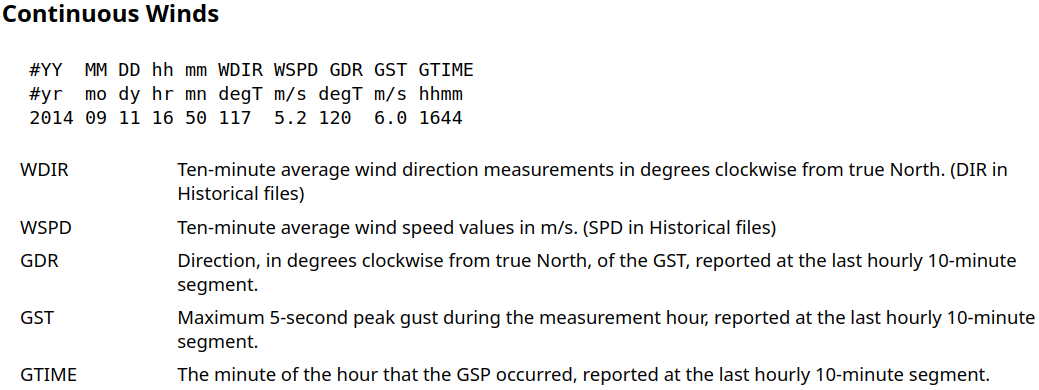
Figure 1. Explanation of variables given by NOAA in relation to wind speed data.

Let's refer to the buoy identified with the code 41001, called "East Hatteras", located at East of Cape Hatteras. The metadata of the buoy are as follows (see here):

Owned and maintained by National Data Buoy Center
3-meter foam buoy
SCOOP payload
34.791 N 72.420 W (34°47'28" N 72°25'12" W)
Site elevation: sea level
Air temp height: 3.7 m above site elevation
Anemometer height: 4.1 m above site elevation
Barometer elevation: 2.7 m above mean sea level
Sea temp depth: 1.5 m below water line
Water depth: 4450 m
Watch circle radius: 4534 yards

Let's look at the data recorded in 1990. The first lines of the file look as shown below:

YY MM DD hh mm    DIR    SPD    GDR    GSP    GMN
90  1     24  15 0        197    10.3     999      99.0    99
90  1     24  15 10      194    11.0     999      99.0    99
90  1     24  15 20      196    9.9       999      99.0    99

Data are available until 2012, with 1994,1995 and 2009 missing. Let's download until year 2006, as 2007 has a different format. Compressed data files may be retrieved and uncompressed in R by the code (tested over Linux Ubuntu, beware of the missing years):

for(i in c(1,2,3,4,7,8,9,10,11,12,13,14,15,16,17))
system(paste("wget https://www.ndbc.noaa.gov/data/historical/cwind/41001c",1989+i,".txt.gz",sep=""))
system("gzip -d *.gz")

The multiple files can be uploaded into R with the following code (beware of the missing years):

for(i in c(1,2,3,4,7,8,9,10,11,12,13,14,15,16,17))
{
assign(paste("wind",1989+i,sep=""),scan(paste("41001c",1989+i,".txt",sep=""), skip =1))
assign(paste("wind",1989+i,sep=""),array(eval(parse(text=paste("wind",1989+i,sep=""))), dim=c(10, length(eval(parse(text=paste("wind",1989+i,sep=""))))/10)))
}

Now let's merge wind speed data together:

windnew=0
for(i in c(1,2,3,4,7,8,9,10,11,12,13,14,15,16,17))
{
windnew=c(windnew, eval(parse(text=paste("wind",1989+i,sep="")))[7,])
}
windnew=windnew[2:length(windnew)] 
windnew1=windnew[windnew!=99]

The maximum value is:

max(windnew1) 

We can plot the time series:

plot(windnew1, type="l", main="Wind speed at East Hatteras",ylab="Wind speed")
grid() 

Note that we excluded missing values, identified with the value 99. The obtained graph is shown in Figure 2.

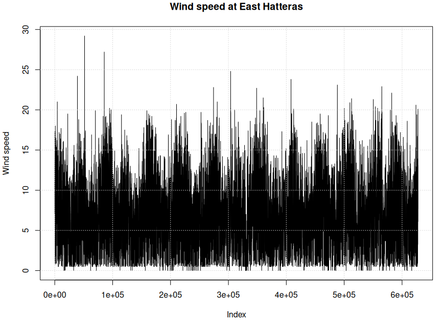
Figure 2: Plot of wind speed at East Hatteras

To better manage the time series let's build the vector of date and time:

year=0
for(i in c(1,2,3,4,7,8,9,10,11,12,13,14,15,16,17))
{
year=c(year, eval(parse(text=paste("wind",1989+i,sep="")))[1,])
}
year=year[2:length(year)]
year1=year[windnew!=99]
month=0
for(i in c(1,2,3,4,7,8,9,10,11,12,13,14,15,16,17))
{
month=c(month, eval(parse(text=paste("wind",1989+i,sep="")))[2,])
}
month=month[2:length(month)]
month1=month[windnew!=99]
day=0
for(i in c(1,2,3,4,7,8,9,10,11,12,13,14,15,16,17))
{
day=c(day, eval(parse(text=paste("wind",1989+i,sep="")))[3,])
}
day=day[2:length(day)]
day1=day[windnew!=99]
hour=0
for(i in c(1,2,3,4,7,8,9,10,11,12,13,14,15,16,17))
{
hour=c(hour, eval(parse(text=paste("wind",1989+i,sep="")))[4,])
}
hour=hour[2:length(hour)]
hour1=hour[windnew!=99]
min=0
for(i in c(1,2,3,4,7,8,9,10,11,12,13,14,15,16,17))
{
min=c(min, eval(parse(text=paste("wind",1989+i,sep="")))[5,])
}
min=min[2:length(min)]
min1=min[windnew!=99] 

Now let's put into a data frame the year and the wind speed:

windspeed=data.frame (
year = year1,
wspeed = windnew1
) 

Be careful: year is expressed with two numbers like "90" before 2000 and then with 4 numbers like "2000" after 1999. Therefore, years are: 90, 91, 92, 93, 96, 97, 98, 99, 2000, 2001, 2002, 2003, 2004, 2005, 2006. Now, let's extract the annual maxima:

annmax=0
for(i in c(1,2,3,4,7,8,9,10,11,12,13,14,15,16,17))
{
year=1989+i
if(year<1999) year=year-1900
annmax=c(annmax, max(windspeed$wspeed[windspeed$year==year]))
}
annmax=annmax[2:length(annmax)]
annmax 

The reason why we are extracting the annual maxima is that this type of observations can reliably be assumed to be outcomes from a population of independent and identically distributed random variables. In fact, annual maxima are widely used for estimation of extreme wind speed (see here).

Extreme estimation will be be dealt with in another lecture.

Last modified on Feb 25, 2026