Running your own climate model

Running your own climate model - Installing WRF on a virtual machine

Here below we present a tutorial to run the WRF model. 

Disclaimer: I am a non expert in climate modelling. The tutorial was compiled by assembling several sources of information. I tried to make a synthesis to provide a guidance to a quick installation and use. I did not go into fine details. You will need to get more information if you want to take full advantage of the capabilities of the WRF model, which is very interesting and up-to-date tool, as you can see below. If you wish additional information please follow the links included in the text. 

Global Climate Models (GCMs)

Global Climate Models (GCMs), also called General Circulation Models, are numerical models that simulate the behavior of the Earth’s climate system. They solve physical equations for how air, water, energy, and momentum move and interact in the atmosphere, ocean, land surface, and cryosphere. 

Key characteristics: 

• Physics-based - GCMs are built on conservation laws: conservation of mass, momentum (Newton’s laws), and energy (thermodynamics and radiative balance). They are not just statistical fits to the past; they try to represent the underlying processes that drive climate.
• 3D and fully coupled - A typical GCM divides the planet into a 3D grid: longitude × latitude × vertical levels. The model steps forward in time (minutes to hours per step), updating temperature, winds, humidity, ocean currents, clouds, etc. Many modern GCMs are “coupled models,” meaning atmosphere, ocean, sea ice, and land all exchange fluxes of heat, moisture, and momentum interactively.
• Forcing and feedbacks - GCMs include external drivers (greenhouse gases, aerosols, solar changes, volcanoes) and internal feedbacks (water vapor, albedo from snow/ice cover, clouds). This means they can be used both to reproduce past climate and to explore “what if” futures.
• Why we use them - To attribute past warming to human vs natural causes, to project future temperature, precipitation, sea level, extremes, To study mechanisms (monsoon shifts, jet stream changes, heatwaves, etc.)

Limitations:

• Resolution is coarse compared to local weather. A typical CMIP6 global model grid is ~100 km, not city scale.
• Sub-grid processes (e.g. convection, cloud microphysics, turbulent mixing, vegetation dynamics) must be parameterized rather than explicitly resolved. Different parameterizations across models → spread in projections. Recent developments - convection permitting models - resolve convective processes but require massive computational resources as they need to run at fine scales.

The WRF model 

The WRF model (quoting from the WRF website) :

 

is a a state of the art mesoscale numerical weather prediction system designed for both atmospheric research and operational forecasting applications. It features two dynamical cores, a data assimilation system, and a software architecture supporting parallel computation and system extensibility. The model serves a wide range of meteorological applications across scales from tens of meters to thousands of kilometers.state of the art mesoscale numerical weather prediction system designed for both atmospheric research and operational forecasting applications. It features two dynamical cores, a data assimilation system, and a software architecture supporting parallel computation and system extensibility. The model serves a wide range of meteorological applications across scales from tens of meters to thousands of kilometers. The effort to develop WRF began in the latter 1990's and was a collaborative partnership of the National Center for Atmospheric Research (NCAR), the National Oceanic and Atmospheric Administration (represented by the National Centers for Environmental Prediction (NCEP) and the Earth System Research Laboratory), the U.S. Air Force, the Naval Research Laboratory, the University of Oklahoma, and the Federal Aviation Administration (FAA).

WRF is a mesoscale numerical weather prediction model, designed to simulate weather and climate at regional to local scales. Therefore, it is primarily a regional climate and weather model. It can be run on limited-area domains (a specific region of interest) with high spatial resolution, from a few kilometers up to hundreds of kilometers. Being a regional model, WRF usually uses boundary conditions from global models or reanalysis data to provide the large-scale forcing. WRF can be adapted for performing global simulations, but it is not typically used for this purpose. Global modelling is typically simulated by using other models, like tne Community Climate System Model (CCSM)

Figure 1. WRF model simulation of Hurricane Rita tracks. The model resolution is 30 km. The colored field shows the lowest sea-level pressure (SLP) recorded during the last 27 hours of a 54 hour control simulation of Rita using LFO (5 class) microphysics and the Kain-Fritsch (KF) convective scheme. The superposed black line traces the model hurricane, which strikes Houston. Also shown are tracks of minimum SLP for runs using the Kessler (warm rain) scheme, the WSM3 simple ice scheme (with the Betts-Miller-Jancic convective scheme), the Kessler with reduced rain fallspeed, and WSM3 with enhanced ice fallspeed. (Bottom): The spread of NHC multi-model ensemble forecast at 06 UTC, 22 September. Note a similar ensemble spread was obtained from a single model simply by varying the model microphysics and convective schemes. Image from Jonathan Vigh, Colorado State University. By Prof. Robert Fovell (UCLA); Dr. Hui Su (JPL), Public domain, via Wikimedia Commons.

Installing WRF on a virtual machine

The WRF model can run in a personal computer, provided the model domain is limited to a reasonable size. It is advisable to run it in a linux operating system in order to maximise computational performances. For the sake of illustrating an example of application, we offer guidelines here below to install WRF over a virtual linux machine.

Why Linux

Linux offers several opportunities and excellent performances for the management of big data, thanks to an efficient use of computational resources. In fact, most of the supercomputers use Linux because it allows for deep optimization to match specific hardware and workload demands, thanks to its open source nature and flexibility. Deep optimisation is necessary for high-performance computing (HPC). The efficiency of Linux allows to run demanding applications even with non-recent personal computers.

Thanks to the recent development of several user interfaces, Linux is also user friendly. Therefore it can be quickly learned and used by non-expert users. There are several distro available (see here for a description of available distro and here for a list). For low performing machines, it is advisable to install a light distro, like Xubuntu or Lubuntu. Linux can be installed as unique operating system or as an alternative to another operating system on the same machine through a dual booting.

Virtual machines  

 A quick possibility is to install linux through a virtual machine. The most used are Vmware and VirtualBox. Be attemptive of the resources that you assign to the virtual machine as this is a key step to ensure that applications run as expected. You may want to see an example of step by step installation of Xubuntu on a VirtualBox virtual machine in this video of one of my lectures.

We select here VirtualBox as virtualisation software. We created a virtual machine with a 50GB hard disk (some more space is recommended). We assigned to the virtual machine 8GB of RAM memory and 4 processors (it should work with less than that). We install the Xubuntu operating system with minimal desktop, automated installation and gave the installation iso file to VirtualBox. The resulting configuration is shown here below.

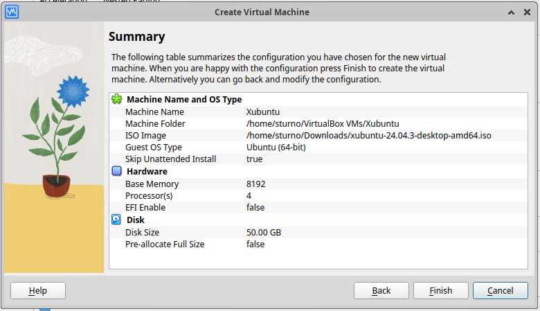
Figure 2. Configuration of the virtual machine in VirtualBox. 

We then selected the option to install Ubuntu. When the machine starts, double click again on the desktop on the install icon. Follow default installation, you will be required to specify the language, your user name, password, keyboard layout, time zone and so forth. 

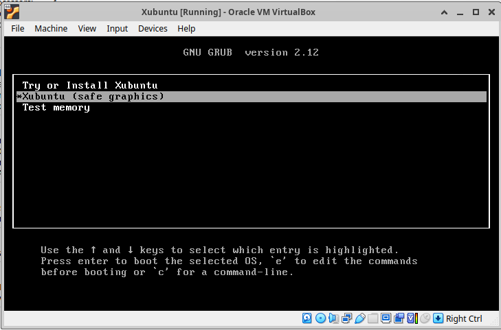
Figure 3. Setting the virtual machine 

You will be required to restart the machine ad the end of the installation. After restarting, click on the menus icon on the upper left and open a terminal.

Then, install Firefox (or other browser) with the command:

Launch firefox and then open the present page so you can copy the commands below. It's now time to install WRF and WPS, the latter being a software for managing WRF input (see Figure 4).

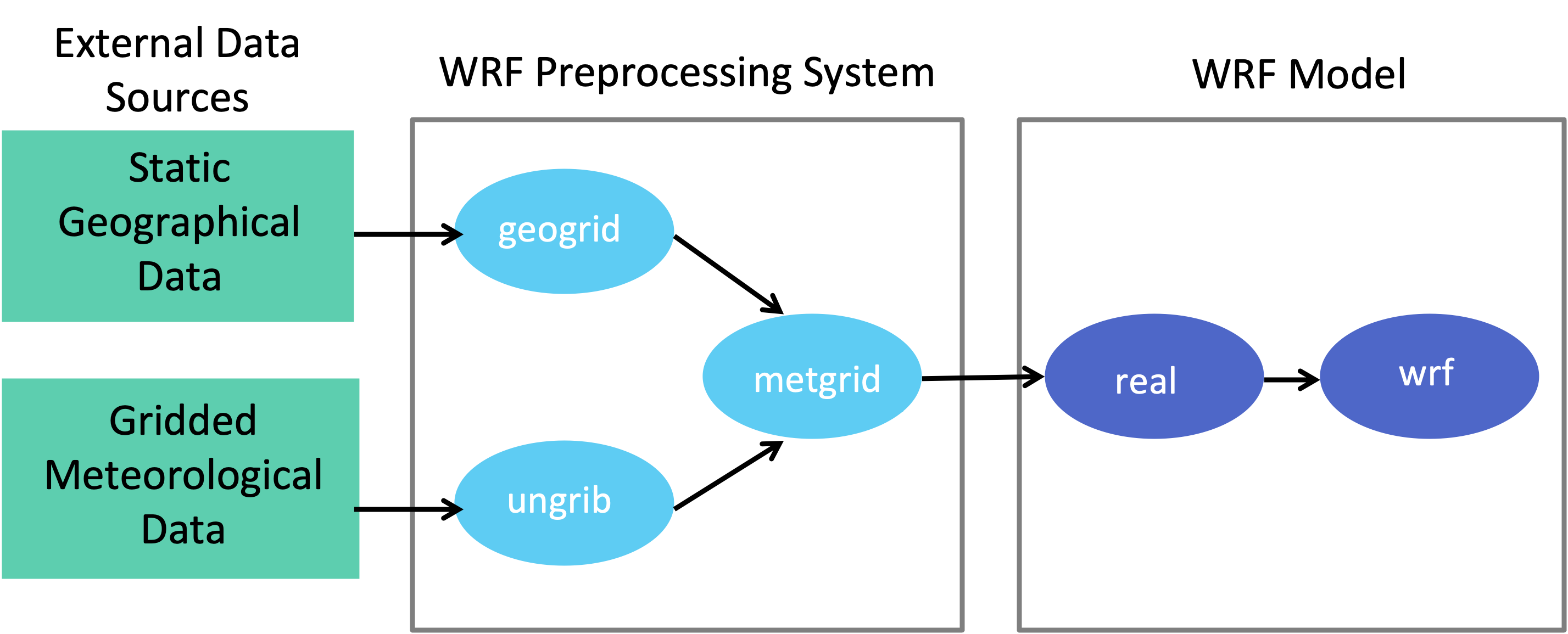
Figure 4.Data flow between WPS and WRF (from NCAR).

Installing WRF 

There a complete guide to install WRF and WPS at NCAR. For getting a ready-to-use solution we suggest to refer to the installation script by Umur Dinç, which installs the needed libraries. The script is written for Debian and Ubuntu based Linux operating systems and is conceived to run on a freshly installed operating system. I used it twice, it got to target successfully in both cases. Please consider that installation takes a long time.

First, download the latest version here I suggest to download the tar file. Then, extract it at the terminal with the command:

Then, get into the directory where the files were extracted and simply run (don't forget to make the installer executable):

After a long time you will get a confirmation of successful install. Now your WRF is ready to be used.

Running WRF on a virtual machine

Initialising WRF - Initialisation data download

From the user guide of WRF:

 

The WRF model has two large classes of simulations that it is able to generate: those with an ideal initialization and those utilizing real data. 

The idealized simulations typically manufacture an initial condition file for the WRF model from an existing 1-D or 2-D sounding and assume a simplified analytic orography.

The real-data cases usually require pre-processing from the WPS package, which provides each atmospheric and static field with fidelity appropriate to the chosen grid resolution for the model. 

The WRF model executable itself is not altered by choosing one initialization option over another (idealized vs. real), but the WRF model pre-processors (the real.exe and ideal.exe programs) are specifically built based upon a user's selection. 

The real.exe and ideal.exe programs are never used together. Both the real.exe and ideal.exe are the programs that are processed just prior to the WRF model run.

The real-data WRF cases are those that have the input data to the “real.exe” program provided by the WRF Preprocessing System (WPS). This data from the WPS was originally generated from a previously-run external analysis or forecast model.

The original data was most-likely in GriB format and was most-likely ingested into the WPS by first ftp'ing the raw GriB data from one of the national weather agencies’ anonymous ftp sites. 

For example, suppose a single-domain WRF forecast is desired, with the following criteria: 

• 2000 January 24 1200 UTC through January 25 1200 UTC
• the original GriB data is available at 6-h increments 

The following coarse-grid files will be generated by the WPS (starting date through ending date, at 6-h increments):

• met_em.d01.2000-01-24_12:00:00.nc · met_em.d01.2000-01-24_18:00:00.nc
• met_em.d01.2000-01-25_00:00:00.nc · met_em.d01.2000-01-25_06:00:00.nc
• met_em.d01.2000-01-25_12:00:00.nc

The convention is to use "met" to signify data that is output from the WPS “metgrid.exe” program and input into the “real.exe” program. The "d01" portion of the name identifies to which domain this data refers, which permits nesting. The next set of characters is the validation date/time (UTC), where each WPS output file has only a single time-slice of processed data. 

The file extension suffix “.nc” refers to the output format from WPS which must be in netCDF for the “real.exe” program. For regional forecasts, multiple time periods must be processed by “real.exe” so that a lateral boundary file is available to the model.

The global option for WRF requires only an initial condition. The WPS package delivers data that is ready to be used in the WRF system by the “real.exe” program.

We focus here on a real case. The starting point for downloading data to initialize WRF is this NCAR page. We went straight to the the NCAR Research Data Archive (NCAR RDA) web site plugged the string "operational model global tropospheric analyses" in the search box. 

Then:

• we selected the NCEP FNL Operational Model Global Tropospheric Analyses, continuing from July 1999; These are (quoting from the web site) ".... on 1-degree by 1-degree grids prepared operationally every six hours. This product is from the Global Data Assimilation System (GDAS), which continuously collects observational data from the Global Telecommunications System (GTS), and other sources, for many analyses. The FNLs are made with the same model which NCEP uses in the Global Forecast System (GFS), but the FNLs are prepared about an hour or so after the GFS is initialized. The FNLs are delayed so that more observational data can be used. The GFS is run earlier in support of time critical forecast needs, and uses the FNL from the previous 6 hour cycle as part of its initialization". Note that a 1-degree by 1-degree resolution is approximately 111 km by 111 km anywhere on Earth (with the actual resolution in kilometers varying with latitude).
• The analyses are available on the surface, at 26 mandatory (and other pressure) levels from 1000 millibars to 10 millibars, in the surface boundary layer and at some sigma layers, the tropopause and a few others. Parameters include surface pressure, sea level pressure, geopotential height, temperature, sea surface temperature, soil values, ice cover, relative humidity, u- and v- winds, vertical motion, vorticity and ozone.
• In the web page we went to "data access";
• We went to the row of "GRIB2 6 HOURLY FILES 2007.12.06 to current";
• We selected "Web download";
• We selected file list,

then getting the web page shown in Figure 5.

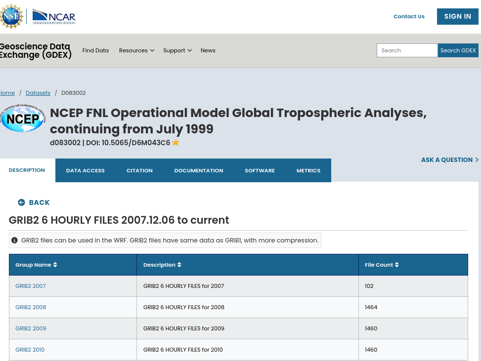
Figure 5. Download of initialisation data

Then, we selected GRIB 2025 and then GRIB2 2025.09 and then selected for download 4 files from fnl_20250901_00_00.grib2 to fnl_20250901_18_00.grib2. We then cliked on "Python download script" thus obtaining a code - downloaded with the name gdex-download.py - that looks like what follows:

 

#!/usr/bin/env python """ 
Python script to download selected files from gdex.ucar.edu.
After you save the file, don't forget to make it executable
i.e. - "chmod 755 <name_of_script>"
"""
import sys, os
from urllib.request import build_opener

opener = build_opener()

filelist = [
 'https://osdf-director.osg-htc.org/ncar/gdex/d083002/grib2/2025/2025.09/fnl_20250901_00_00.grib2',
 'https://osdf-director.osg-htc.org/ncar/gdex/d083002/grib2/2025/2025.09/fnl_20250901_06_00.grib2',
 'https://osdf-director.osg-htc.org/ncar/gdex/d083002/grib2/2025/2025.09/fnl_20250901_12_00.grib2',
 'https://osdf-director.osg-htc.org/ncar/gdex/d083002/grib2/2025/2025.09/fnl_20250901_18_00.grib2'
]

for file in filelist:
   ofile = os.path.basename(file)
   sys.stdout.write("downloading " + ofile + " ... ")
   sys.stdout.flush()
   infile = opener.open(file)
   outfile = open(ofile, "wb")
   outfile.write(infile.read())
   outfile.close()
   sys.stdout.write("done\n")

Then in the terminal we need to run:

thus downloading the files, that need to be moved into the directory Build_WRF/INPUT_DATA that you need to create beforehand into the directory Build_WRF, that was created by the installation file.

Initialising WRF - WPS preprocessing

We first need to give the details of our simulation in the file "namelist.wps", that is located in the directory WPS-4.6.0. To do so, we suggest to first install the text editor "Kate" (or another one of your choice) by the terminal command:

and then

For a detailed explanation of the options for the file please see here.

First, we need to set the number of domains. If we want to simulate in nested domains, we need more than one domain. For this example we select only one domain.

Then, we need to set start date and end date. For this simulation we decided to run the model for 18 hours only, so the dates read as:

 

start_date = '2025-09-01_00:00:00',
end_date   = '2025-09-01_18:00:00',

We need to set dates that correspond to the timing of the downloaded initialisation files, as done for the dates above (we downloaded 4 files corresponding to 12AM, 6AM, 12PM, 6PM).

The time interval corresponds to the number of seconds in the time step of six hours.

Regarding the coordinates to include in the file under the &geogrid sesction, you may use the domain analyser available here. Be careful to cut and past from the domain analyser to namelist.wps only the domain data.

We want here a domain close to Bologna and therefore used the following settings:

 

&geogrid
parent_id         =   1,
parent_grid_ratio =   1,
i_parent_start    =   1,
j_parent_start    =   1,
e_we              =  14,
e_sn              =  12,
geog_data_res = 'default',
dx = 15000,
dy = 15000,
map_proj = 'lambert',
ref_lat              = 44.569
ref_lon              = 11.576
truelat1             = 44.461
truelat2             = 44.461
stand_lon            = 11.349
geog_data_path = '../WPS_GEOG/'

We are now ready to run WPS with the following sequence of commands:

For geogrid and ungrib you should get a message like "SUCCESS!" at the end of the run.

Running WRF

We are now ready to launch WRF. We should go into the directory WRF-4.6.1-ARW/run and then first edit the file "namelist.input" to provide simulation information. We need to set the following parameters:

• run days, hours, minutes, seconds. In this example we are running the simulation for 18 hours, so let's set run_hours=18 and days, minutes, seconds to 0;
• start and end year,  month, day, hour, like in the file namelist.wps;
• interval_seconds: the same as in namelist.wps (21200 in our case);
• time_step: the maximum value is given by max(Dx,Dy)/1000 * 6. In our case, Dx=Dy=15000, so we set time_step=90;
• max_dom as in namelist.wps;
• e_we, e_sn as in namelist.wps;

Now we need to copy the met_em* files created by WPS in the directory WPS-4.5.0 into the subdirectory "run" of the directory WRF-4.6.1, with a file manager. The sequence of commands to run WRF is:

Parameter "np" indicates the number of processors. At the end of the simulation we can test success by

which should result in one or more outcomes like "SUCCESS". Also, make sure you have all the wrfout* files you anticipated having, that is, one per each simulation hour. If so, the run was successful, and you are ready to do analysis for your project.

If simulation was not successful, the above check will give you detailed information on the error. Most likely there are parameters that need to be adjusted in namelist.wps or namelist.input

Visualisation of results

Outfiles are in a conventional format "nc" format. To analyse the results, there are several available options. We decided to use Anaconda, which needs to be installed in the virtual machine. 

To install Anaconda, we selected the option of installing Miniconda: go here and select the appropriate 64-bit bash installer (please note: you need to register for free to download, or access through Google or other). Then, go to the terminal, make the installer executable and run it by:

Reply "yes" to all questions. When the installation is finished, close and reopen the terminal for changes to take effect. You can test installation quickly by typing the following from the terminal window:

This should echo something like "conda 4.6.2" (Note: you can also get the conda command line by downloading and installing Anaconda). To activate conda digit:

then install ncl through

You will need to run the "source activate ncl_stable" command every time you log out and log back in. 

To explore the content of the file we can use terminal commands, for instance for knowing the name of variables, or can use visualisation tools. There is a very good tutorial here, with examples of case studies.

From the terminal, to know the name of variables we can use:

where "d01_2025-09-01_00:00:00" is the output file we want to see.

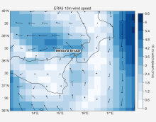
A first very useful visualisation tool is ncview, that can be installed from the terminal:

and then run from the terminal again:

therefore getting what is displayed in Figure 6 below.

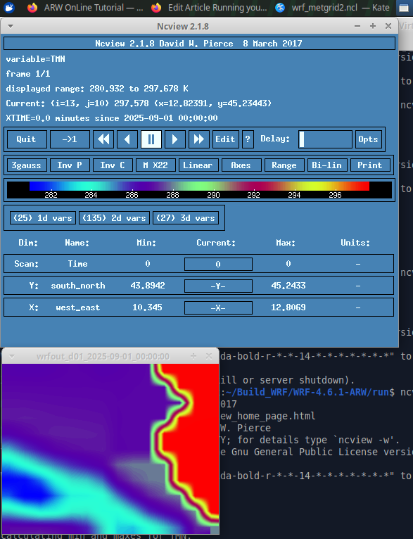
Figure 6. Screenshot from Ncviewer.

A second option to visualisation is to upload a ncl script. There are many script available here. An example is the script below (note the file name in the code, and note that the script can be downloaded here), which is uploaded with the instruction:

where "namefile.ncl" corresponds to the file name you selected (with extension "ncl"). The script to be stored into "namefile.ncl"  is:

 

;   Example script to plot a variable from a single output WRF file
;   By Alberto, November 2025, template taken from https://www2.mmm.ucar.edu/wrf/OnLineTutorial/Graphics/NCL/Examples/BASIC/wrf_metgrid2.ncl
load "$NCARG_ROOT/lib/ncarg/nclscripts/csm/gsn_code.ncl"
load "$NCARG_ROOT/lib/ncarg/nclscripts/wrf/WRFUserARW.ncl" 
begin
;
 a = addfile("wrfout_d01_2025-09-01_00:00:00","r")  ; Open a file
; We generate plots, but what kind do we prefer?
 type = "x11"
; type = "pdf"
; type = "ps"
; type = "ncgm"
 wks = gsn_open_wks(type,"plt_metgrid_2")
 res = True                           ; Set up some basic plot resources
 res@MainTitle = "Output WRF file"
 res@Footer = False
 pltres = True
 mpres = True
; Get 2m temperature
 t2 = wrf_user_getvar(a,"T2",0)    ; Get T2 from file
; Example to get total rain
;  rainnc = wrf_user_getvar(a,"RAINNC",0)    ; Get RAINNC from file
;  rainc = wrf_user_getvar(a,"RAINC",0)    ; Get RAINC from file
;  rain_tot=rainnc+rainc
   opts = res
   opts@cnFillOn            = True
   contour = wrf_contour(a,wks,t2,opts)
;    contour = wrf_contour(a,wks,rainnc+rainc,opts)
   plot = wrf_map_overlays(a,wks,(/contour/),pltres,mpres)
end

The above code gives the picture displayed in Figure 7.

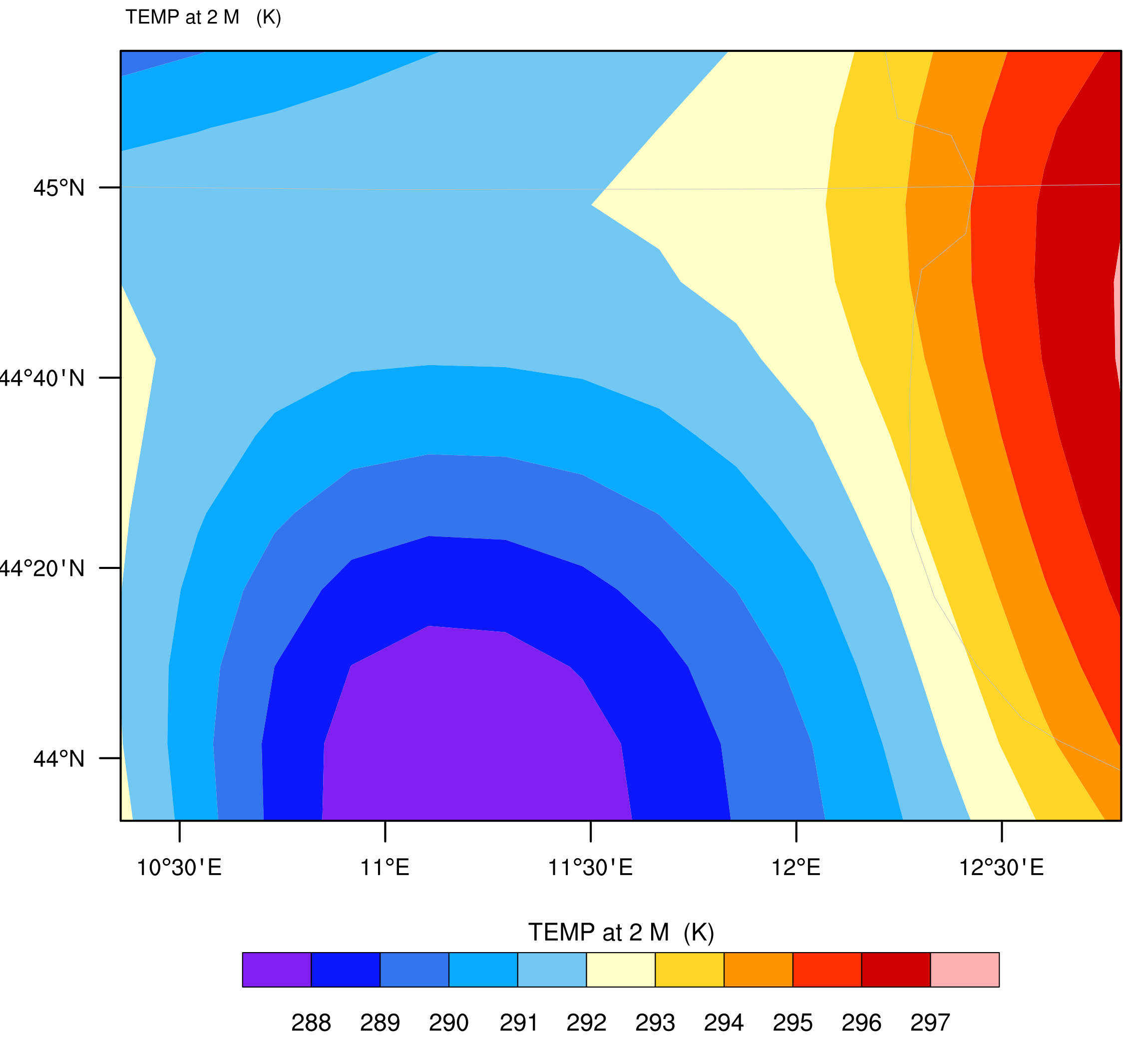
Figure 7. Graphical representation of 2m elevation air temperature obtained with this script. 

More sophisticated outputs - including animations from the sequence of output files - can be produced by following the tutorial here.

Note: the above example refers to simulation of past climate. To simulate future climate you need to download proper initial and boundary conditions, which are determined for the different emission scenarios. This information for future climate can be downloaded from the NCAR web site. 

References 

List to be compiled

Tutorial to be completed

Last modified on November 20, 2025